Trying to calculate proper shading
It all started with the following statement: "my renders are too slow". There were three issues as the root case: osm-carto had become more complex (nothing I can do there), my compute resources were too nimble (but upgrading them would cost money I don't want to spend in just one hobby) and the terrain rasters were being reprojected all the time.
My style uses three raster layers to provide a sense of relief: one providing height tints, one enhancing that color on slopes and desaturating it on valleys, and a last one providing hill shading. All three were derived from the same source DEM, which is projected in WGS 84 a.k.a. EPSG 4326. The style is of course in Pseudo/Web Mercator, a.k.a. EPSG 3857; hence the constant reprojection.
So my first reaction was: reproject first, then derive the raster layers. This single step made it all hell break loose.
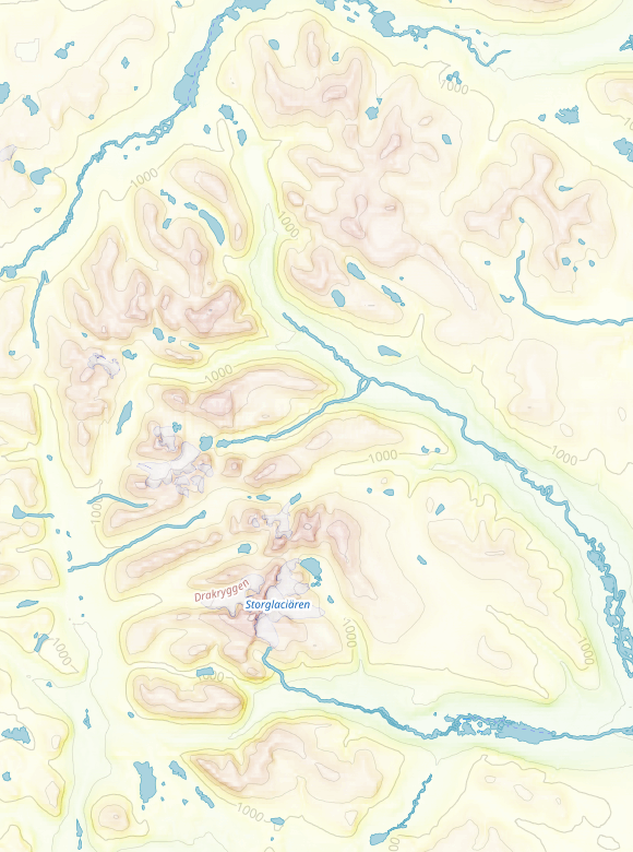
I usually render Europe. It's the region where I live and where I most travel to. I'm using relief layers because I like mountains, so I'm constantly checking how they look. And with this change, the mountains up North (initially was around North Scandinavia) looked all washed out:
The reason behind this is that GDAL's hill and slope shading algorithms don't take in account the projection, but just use pixel values as present in the dataset and the declared pixel size. The DEMs I'm using are of a resolution of 1 arc second per pixel. WGS84 assumes a ellipsoid of 6_378_137m of radius (plus a flattening parameter which we're going to ignore), which means a circumference at the Equator of:
In [1]: import math
In [2]: radius = 6_378_137  # in meters
In [3]: circunf = radius * 2 * math.pi  # 2πr
In [4]: circunf
Out[4]: 40_075_016.68557849  # in meters
One arc second is hence this 'wide':
In [5]: circunf / 360 / 60 / 60
Out[5]: 30.922080775909325  # in meters
In fact the DEMs advertises exactly that:
mdione@diablo:~/src/projects/osm/data/height/mapzen$ gdalinfo N79E014.hgt
Size is 3601, 3601
Coordinate System is:
GEOGCRS["WGS 84",
    DATUM["World Geodetic System 1984",
        ELLIPSOID["WGS 84",6378137,298.257223563,
            LENGTHUNIT["metre",1]]],
    PRIMEM["Greenwich",0,
        ANGLEUNIT["degree",0.0174532925199433]],
    CS[ellipsoidal,2],
        AXIS["geodetic latitude (Lat)",north,
            ORDER[1],
            ANGLEUNIT["degree",0.0174532925199433]],
        AXIS["geodetic longitude (Lon)",east,
            ORDER[2],
            ANGLEUNIT["degree",0.0174532925199433]],
    ID["EPSG",4326]]
Pixel Size = (0.000277777777778,-0.000277777777778)
Well, not exactly that, but we can derive it 'easily'. Deep down there, the
declared unit is degree (ignore the metre in the datum; that's the unit for
the numbers in the ELLIPSOID) and its size in radians (just in case you aren't
satisfied with the amount of conversions involved, I guess). The projection declares
degrees as the unit of the projection for both axis, and the pixel size is declared in the units of the
projection, and 1 arc second is:
In [6]: 1 / 60 / 60  # or 1/3600
Out[6]: 0.0002777777777777778  # in degrees
which is exactly the value declared in the pixel size12. So one pixel is one arc second and one arc second is around 30m at the Equator.
The 'flatness' problem arises because all these projections assume all latitudes are of the
same width; for them, a degree at the Equator is as 'wide' as one at 60°N, which is not; in reality,
it's twice as wide, because the width of a degree decreases with the cosine of the latitude and
math.cos(math.radians(60)) == 0.5. The
mountains we saw in the first image are close to 68N; the cosine up there is:
In [7]: math.cos(math.radians(68))
Out[7]: 0.37460659341591196
So pixels up there are no longer around 30m wide, but only about
30 * 0.37 ≃ 11 # in meters!
How does this relate to the flatness? Well, like I said, GDAL's algorithms use the declared pixel size everywhere, so at f.i. 68°N it thinks the pixel is around 30m wide when it's only around 11m wide. They're miscalculating by a factor of almost 3! Also, the Mercator projection is famous for stretching not only in the East-West direction (longitude) but also in latitude, at the same pace, based on the inverse of the cosine of the latitude:
stretch_factor = 1 / math.cos(math.radians(lat))
So all the mountains up there 'look' to the algorithms as 3 times wider and 'taller' ('tall' here means in the latitude, N-S direction, not height AMSL), hence the washing out.

In that image we have an original mountain 10 units wide and 5 units tall; but gdal
thinks it's 20 units wide, so it looks flat.
Then it hit me: it doesn't matter what projection you are using, unless you calculate slopes and hill shading on the sphere (or spheroid, but we all want to keep it simple, right? Otherwise we wouldn't be using WebMerc all over :), the numbers are going to be wrong.
The Wandering Cartographer
mentions this
and goes around the issue by doing two things: Always using DEMs where the units
are meters, and always using a local projection that doesn't deform as much. He can do that
because he produces small maps. He also concedes he is
using the 111_120 constant
when the unit is degrees.
I'm not really sure about how that number is calculated, but I suspect that it
has something to do with the flattening parameter, and also some level of
rounding. It seems to have originated from
gdaldem's manpage
(search for the -s option). Let's try something:
In [8]: m_per_degree = circunf / 360
In [9]: m_per_degree
Out[9]: 111_319.49079327358  # in meters
That's how wide is a degree is at the Equator. Close enough, I guess.
But for us world-wide, or at least continent-wide webmappers like me, those suggestions are not enough; we can't choose a projection that doesn't deform because at those scales they all forcibly do, and we can't use a single scaling factor either.
gdal's algorithm
uses the 8 neighboring pixels of a pixel to determine slope and aspect. The slope
is calculated on a sum of those pixels' values divided by the cell size. We can't change the
cell size that gdal uses, but we can change the values :) That's the third triangle up there: the algorithm
assumes a size for the base that it's X times bigger than the real one, and we just make the
triangle as many times taller. X is just 1 / math.cos(math.radians(lat)).
If we apply this technique at each DEM file individually, we have to chose a latitude for it. One option is
to take the latitude at the center of the file. It would make your code from more
complicated, specially if you're using bash or, worse, make because you have to pass a
different value for -s, but you can always use a little bit of Python or any other high level,
interpreted language.
But what happens at the seams where one tile meets another? Well, since each file has it's own latitude, two neighbouring values, one in one DEM file and the other in another, will have different compensation values. So, when you jump from a ~0.39 factor to a ~0.37 at the 68° of latitude, you start to notice it, and these are not the mountains more to the North that there are.
The next step would be to start cutting DEM tiles into smaller ones, so the 'jumps' in between are less noticeable... but can we make this more continuous-like? Yes we can! We simply compensate each pixel based on its latitude.
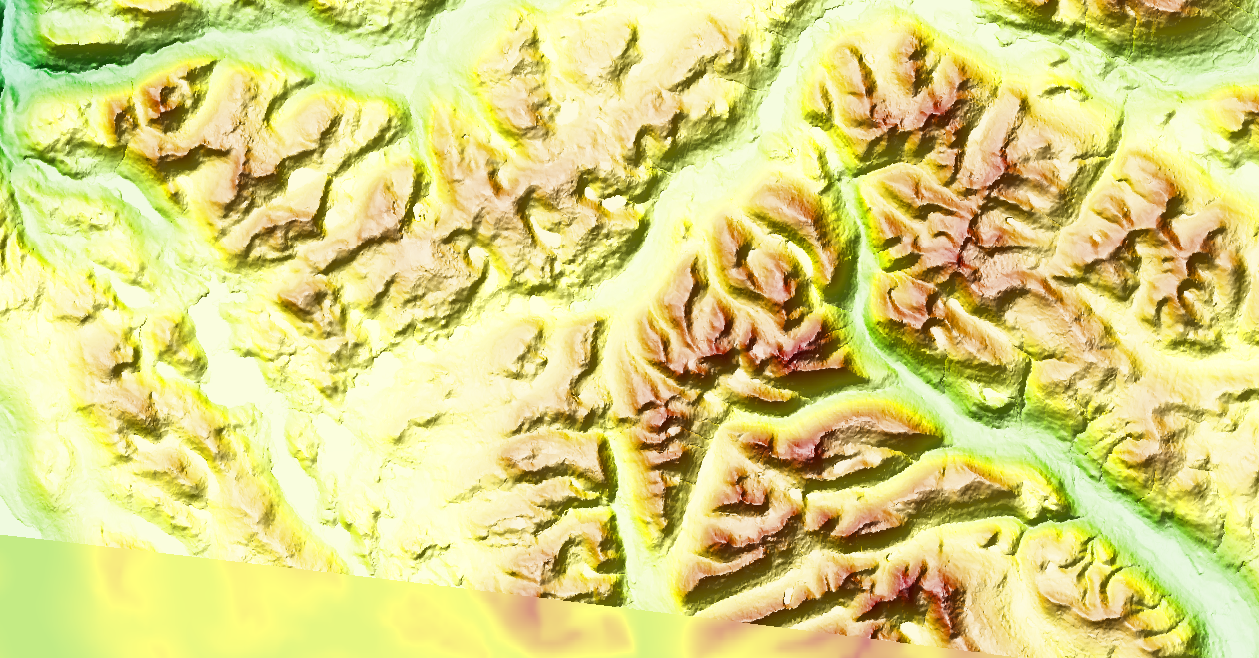
This image cheats a little; this one is based on EU-DEM and not mapzen like the original. You can see where the DEM file ends because the slope and hillshading effects stop at the bottom left. I still have to decide which dataset I will use; at some point I decided that EU-DEM is not global enough for me, and that it's probably better to use a single dataset (f.i. mapzen) than a more accurate but partial one, but since I usually render the regions I need, I might as well change my workflow to easily change the DEM dataset.
This approach works fine as shown, but has at least one limitation. The data type used in those TIFFs
is Int16. This means signed ints 16 bits wide, which means values can go between -32768..32767.
We could only compensate Everest up to less than 4 times, but luckily we don't have to; it
would have to be at around 75° of latitude before the compensated value was bigger than the
maximum the type can represent. But at around 84° we get a compensation of 10x
and it only gets quickly worse from there:
75:  3.863
76:  4.133
77:  4.445
78:  4.809
79:  5.240
80:  5.758
81:  6.392
82:  7.185
83:  8.205
84:  9.566
85: 11.474
86: 14.336
87: 19.107
88: 28.654
89: 57.299  # we don't draw this far, the cutout value is around 85.5 IIRC
90: ∞       # :)
The solution could be to use a floating point type, but that means all calculations would
be more expensive, but definitely not as much as reprojecting on the fly. Or maybe we can use
a bigger integer type. Both solutions would also use more disk space and require more memory.
gdal currently supports band types of Byte, UInt16, Int16, UInt32, Int32, Float32, Float64,
CInt16, CInt32, CFloat32 and CFloat64 for reading and writing.
Another thing is that it works fine and quick for datasets like SRTM and mapzen because I can compensate whole raster lines in one go as all its pixels have the same latitude, but for EU-DEM I have to compensate every pixel and it becomes slow. I could try to parallelize it (I bought a new computer which has 4x the CPUs I had before, and 4x the RAM too :), but I first have to figure out how to slowly write TIFFS; currently I have to hold the whole output TIFF in memory before dumping it into a file.
Here's the code for pixel per pixel processing; converting it to do row by row for f.i. mapzen makes you actually remove some code :)
#! /usr/bin/env python3

import sys
import math

import rasterio
import pyproj
import numpy

in_file = rasterio.open(sys.argv[^1])
band = in_file.read(1)  # yes, we assume only one band

out_file = rasterio.open(sys.argv[^2], 'w', driver='GTiff',
                         height=in_file.height, width=in_file.width,
                         count=1, dtype=in_file.dtypes[0],
                         crs=in_file.crs, transform=in_file.transform)
out_data = []

transformer = pyproj.Transformer.from_crs(in_file.crs, 'epsg:4326')

# scan every line in the input
for row in range(in_file.height):
    if (row % 10) == 0:
        print(f"{row}/{in_file.height}")

    line = band[row]

    # EU-DEM does not provide 'nice' 1x1 rectangular tiles,
    # they use a specific projection that become 'arcs' in anything 'rectangular'

    # so, pixel by pixel
    for col in range(in_file.width):
        # rasterio does not say where do the coords returned fall in the pixel
        # but at 30m tops, we don't care
        y, x = in_file.xy(row, col)

        # convert back to latlon
        lat, _ = transformer.transform(y, x)

        # calculate a compensation value based on lat
        # real widths are pixel_size * cos(lat), we compensate by the inverse of that
        coef = 1 / math.cos(math.radians(lat))

        line[col] *= coef

    out_data.append(line)

# save in a new file.
out_file.write(numpy.asarray(out_data, in_file.dtypes[^0]), 1)
That's it!
