I forgot to mention: I did a couple of ayrton releases, one more than a month ago and another a couple of days ago. One thing to notice is that even when 0.4.4 introduces an incompatible change (source() is no more), I didn't bump the minor or major version, as the level of usage is practically null. Here's the combined changelog:

• source() is out. use python's import system.
• Support executing foo.py().
• Let commands handle SIGPIE and SIGINT. Python does funky things to them.
• for line in foo(): ... forces Capture'ing the output.
• Fix remote() a little. The API stills sucks.
• Fix remote() tests.

Get it on github or pypi!

So it's been a long while that I talked about my quest towards the perfect map for in-car navigation and general orientation. This post is to fix that.

I started with marble, monav and OSM tiles. The tiles proved inefficient for in-car navigation because of the non-contrasting palette, which makes differentiating ways from blocks very difficult in the sunlight. Then I switched to creating maps with CloudMade, which at the beginning seemed enough, but then I noticed that the solution was not complete, as it lacked some features (in OSM terms) that couldn't be mapped. When I started to look for alternatives, I found a site that showed TileMill, which can use OSM data from a database, and specially its ability to create relief maps, with altitude coloring, slope and hillshading. I was doomed :)

I started exploring the relief part. relief data is available from several sources, the most prominent being the ones derived from the Shuttle Radar Topography Mission, like CGIAR-CSI or Jonathan de Ferranti. Discussing with a friend, he told me to stick to the first ones, as de Ferranti's data has been smoothed by hand and is not always the best. Also, his several sources have incompatible licenses, so it should be unusable. With this data I also generated contour lines, which you will recognize from topographic maps.

The next step is how to use OSM data. I started using GeoFabrik's extracts, first importing the data into a database, but this takes a lot of time, memory and disk space. I switched to the shapefiles, but this introduced several problems. First, the sum of the data contained in the several shapefiles for a region (landuse, natural, places, points, railways, roads and waterways) are not the entire set of data; for instance, all data related to ski lifts is not there. I wanted those. So I reluctantly reverted to importing the data in a database.

Then there's the problem of rendering a usable map. Both TileMill and OSM render the tiles using Mapnik, which implements the so called Painter's algorithm: you define layers and they're 'painted' from bottom up, one on top of the other. So, what do you put in a layer? You define a data source, which is a select in the database, and you link it to a style. A style defines several rules, which can provide extra filters (which technically you could do in the database, but simplifies the data source definitions), min and/or max scales (related to zoom levels) and how to paint them: fill a polygon, draw a line, put a symbol, write some text, etc.

Clearly, just like that, the complexity is big. Defining if a feature appears in a zoom level or not and how, specially if it changes between zoom levels, is quite complex. Then you have more factors: putting borders to a line is actually implemented as drawing two lines, one thicker, defining the borders, and then a thinner one on top of it, defining the inner part, done in two different layers. This is called casing. Also, think that you have to change the casing and the fill color when there is a tunnel or add an extra casing (layer) for a bridge, and even when there are several bridges on top of each other (think of complex highway junctions; implementet with more layers)! TileMill proved to be good for testing, but this level of nitpicking was too much for it.

For a while I flirted with the idea of generating the Mapnik input file with a structural description of what I wanted, but I aborted it before it became a monster. I learned something from Frankenstein!

So, why not come full circle and take a look at how the OSM tiles are generated? This was definitely the right move. Instead of trying to mimic the complex set of rules and layers that make OSM tiles perfect, just edit the xml files to take out uninteresting data, modify some zoom levels here and there to make some things appear sooner (I'm very interested in gas stations, hospitals, parkings, archaeological sites and viewpoints), and edit the colors. I can even export what I have done in TileMill to a Mapnik project, extract the part where a define the relief layers and add them as the background.

So the final setup is as following:

• Use elevation information from CGIAR-CSI, process them as TileMill says.
• Use Geofabrik's pbf extracts; import them in a PostGis Database as per this page in OSM's wiki.
• Use TileMill for initial designing, specially about color changes.
• Modify osm.xml by hand, picking out what's not wanted, changing zoom levels for some stuff.
• Use a script to extract colors and line widths from osm.xml; use the colors designed with TileMill.
• Use a modified version of generate_tiles.py to render big areas or special cities.

I almost have it finished with the scripts that allows me to iterate over the last two steps without much hand intervention (except tweaking the values, of course). When I'm done I'll publish it, then clean it up, then republish :)

As I mentioned in one of my lasts posts about it, I started using SRTM 1 arc data for rendering my maps. So far, with the 3 arc dataset, I was able to generate a huge image by stitching the tiles with gdal_merge.py, then generating the 3 final images (height, slope and hill shade) plus one intermediary for the slope, all with gdaldem. Now this is no longer possible, as the new dataset is almost 10x the old one, so instead of going that way, I decided to try another one.

With gdalbuildvrt it is possible to generate an XML file that 'virtually' stitches images. This means that any attempt to access data through this file will actually make the library (libgdal) to find the proper tile(s) and access them directly.

So now the problem becomes processing each tile individually and then virtual stitching them. The first part is easy, as I just need to do the same I was doing to the huge stitched image before. I also took the opportunity to use tiled files, which instead of storing the image one scan line at a time (being 1 arc second resolution, each scan line has 3601 pixels; the extra one is for overlapping with the neighbors), it stores the file in 256x256 sub-tiles, possibly (that is, no tested) making rendering faster by clustering related data closer. The second step, with gdalbuildvrt, should also be easy.

The first block on the way is the fact that SRTM tiles above 50°N are only 1801 pixels wide, most posibly because it makes no sense anyways. This meant that I had to preprocess the original tiles so libgdal didn't have to do the interpolation at render time (in fact, it already has to do it once while rendering, using the lanczos scaling algorithm). This was done with gdalwarp.

The second one came from slope and hill shading tiles. As the algortihm goes, it generates some 'fade out' values in the edges, and when libgdal was stitching them, I could see it as a line in the seam. This was fixed by passing -compute_edges to gdaldem.

Finally, for some reason gdalbuildvrt was generating some very strange .vrt files. The format of these files is more or less the following:

• For each band in the source tiles it creates a band in the result.
  • For each source tile, it describes:
    • The source file
    • The source band
    • The size and tiling of the source (3601², 256²)
    • The rectangle we want from the source (0², 3601²)
    • The rectangle in the result (x, y, 3601²)

The problem I saw was some weird declararions of the rectangles in the result, where the coordinates or the sizes didn't match what I expected. I will try to figure this out with the GDAL poeple in the following weeks, but first I want to make sure that the source tiles are easily downloadable (so far I have only found download options through USGS' EarthExplorer, which requires you to be logged in in order to download tiles, which means that it is not very scriptable, so not very reproducible).

So for the moment I'm using my own .vrt file generator, completely not generic enough for release, but soon. I also took the opportunity to make the rectangles in the result non-overlapping, being just 3600² in size. I know that the generated file works because I'm also generating smaller samples of the resulting layers (again, height, slope and hill shading) for rendering smaller zoom levels.

The only remaining question about huge DEM datasets is contour generation. So far I had just generated contour lines for each tile and lived with the fact that they too look ugly at the seams.

First: one thing I didn't do in previous post was to show the final tables and sizes. Here it is:

 Schema |        Name        | Type  | Owner  |  Size   | Description
--------+--------------------+-------+--------+---------+-------------
 public | geography_columns  | view  | mdione | 0 bytes |
 public | geometry_columns   | view  | mdione | 0 bytes |
 public | planet_osm_line    | table | mdione | 11 GB   |
 public | planet_osm_point   | table | mdione | 2181 MB |
 public | planet_osm_polygon | table | mdione | 23 GB   |
 public | planet_osm_roads   | table | mdione | 2129 MB |
 public | raster_columns     | view  | mdione | 0 bytes |
 public | raster_overviews   | view  | mdione | 0 bytes |
 public | spatial_ref_sys    | table | mdione | 3216 kB |

 Schema |            Name             | Type  | Owner  |       Table        |  Size   | Description
--------+-----------------------------+-------+--------+--------------------+---------+-------------
 public | planet_osm_line_index       | index | mdione | planet_osm_line    | 4027 MB |
 public | planet_osm_point_index      | index | mdione | planet_osm_point   | 1491 MB |
 public | planet_osm_point_population | index | mdione | planet_osm_point   | 566 MB  |
 public | planet_osm_polygon_index    | index | mdione | planet_osm_polygon | 8202 MB |
 public | planet_osm_roads_index      | index | mdione | planet_osm_roads   | 355 MB  |
 public | spatial_ref_sys_pkey        | index | mdione | spatial_ref_sys    | 144 kB  |

The first thing to notice is that none of the intermediate tables are created nor their indexes, but also all the _pkey indexes are missing.

What I did in my previous post was to say that I couldn't update because the intermediate tables were missing. That was actually my fault. I didn't read carefully osm2psql's manpage, so it happens that the --drop option is not for dropping the tables before importing but for dropping the intermediate after import.

This means I had to reimport everything, and this time I made sure that I had the memory consumption log. But first, the final sizes:

 Schema |        Name        |   Type   | Owner  |    Size    | Description
--------+--------------------+----------+--------+------------+-------------
 public | contours           | table    | mdione | 21 GB      |
 public | contours_gid_seq   | sequence | mdione | 8192 bytes |
 public | geography_columns  | view     | mdione | 0 bytes    |
 public | geometry_columns   | view     | mdione | 0 bytes    |
 public | planet_osm_line    | table    | mdione | 11 GB      |
 public | planet_osm_nodes   | table    | mdione | 16 kB      |
 public | planet_osm_point   | table    | mdione | 2181 MB    |
 public | planet_osm_polygon | table    | mdione | 23 GB      |
 public | planet_osm_rels    | table    | mdione | 871 MB     |
 public | planet_osm_roads   | table    | mdione | 2129 MB    |
 public | planet_osm_ways    | table    | mdione | 42 GB      |
 public | raster_columns     | view     | mdione | 0 bytes    |
 public | raster_overviews   | view     | mdione | 0 bytes    |
 public | spatial_ref_sys    | table    | mdione | 3216 kB    |

 Schema |           Name           | Type  | Owner  |       Table        |  Size   | Description
--------+--------------------------+-------+--------+--------------------+---------+-------------
 public | contours_height          | index | mdione | contours           | 268 MB  |
 public | contours_pkey            | index | mdione | contours           | 268 MB  |
 public | contours_way_gist        | index | mdione | contours           | 1144 MB |
 public | planet_osm_line_index    | index | mdione | planet_osm_line    | 4022 MB |
 public | planet_osm_line_pkey     | index | mdione | planet_osm_line    | 748 MB  |
 public | planet_osm_nodes_pkey    | index | mdione | planet_osm_nodes   | 16 kB   |
 public | planet_osm_point_index   | index | mdione | planet_osm_point   | 1494 MB |
 public | planet_osm_point_pkey    | index | mdione | planet_osm_point   | 566 MB  |
 public | planet_osm_polygon_index | index | mdione | planet_osm_polygon | 8207 MB |
 public | planet_osm_polygon_pkey  | index | mdione | planet_osm_polygon | 1953 MB |
 public | planet_osm_rels_idx      | index | mdione | planet_osm_rels    | 16 kB   |
 public | planet_osm_rels_parts    | index | mdione | planet_osm_rels    | 671 MB  |
 public | planet_osm_rels_pkey     | index | mdione | planet_osm_rels    | 37 MB   |
 public | planet_osm_roads_index   | index | mdione | planet_osm_roads   | 358 MB  |
 public | planet_osm_roads_pkey    | index | mdione | planet_osm_roads   | 77 MB   |
 public | planet_osm_ways_idx      | index | mdione | planet_osm_ways    | 2161 MB |
 public | planet_osm_ways_nodes    | index | mdione | planet_osm_ways    | 52 GB   |
 public | planet_osm_ways_pkey     | index | mdione | planet_osm_ways    | 6922 MB |
 public | spatial_ref_sys_pkey     | index | mdione | spatial_ref_sys    | 144 kB  |

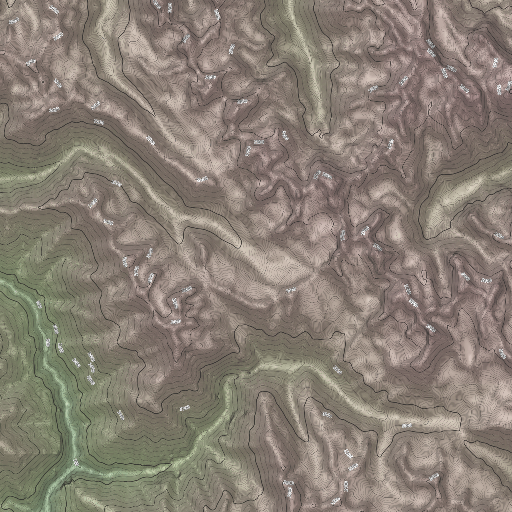
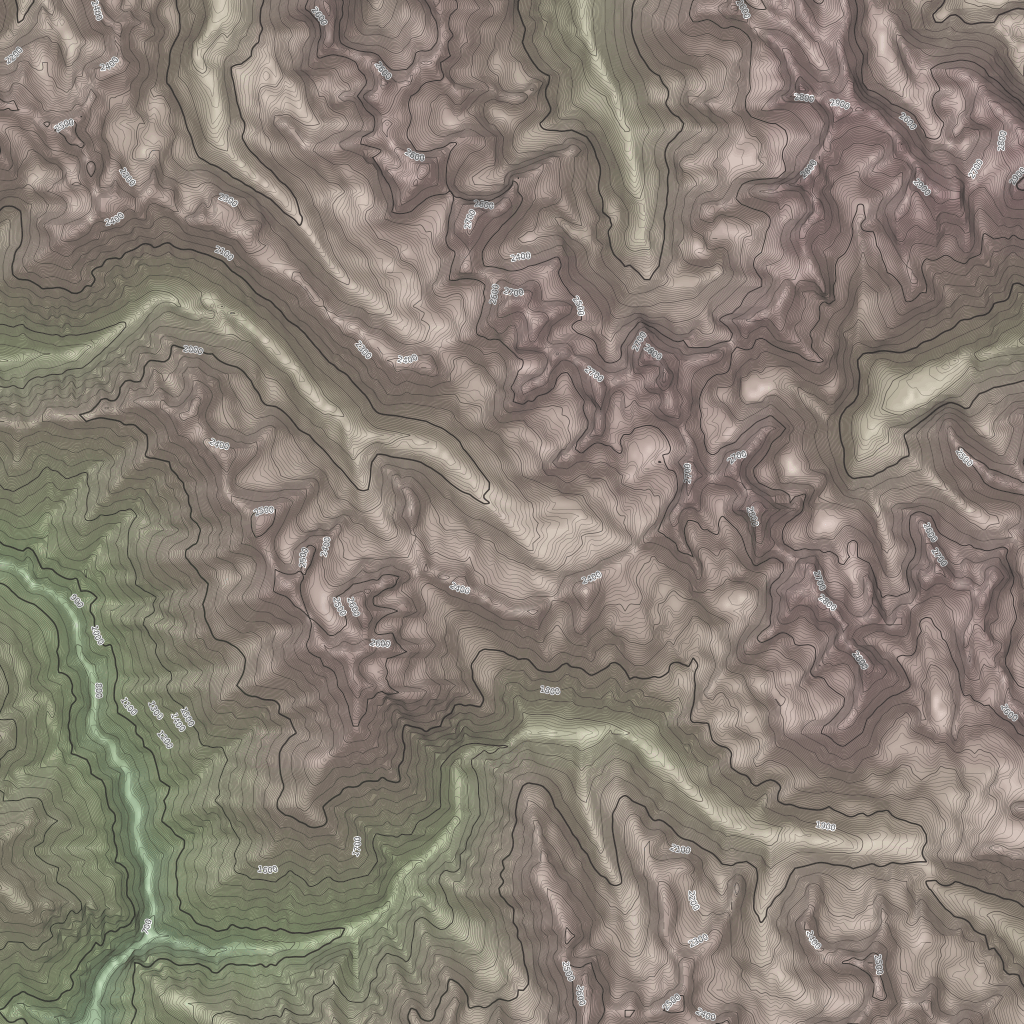
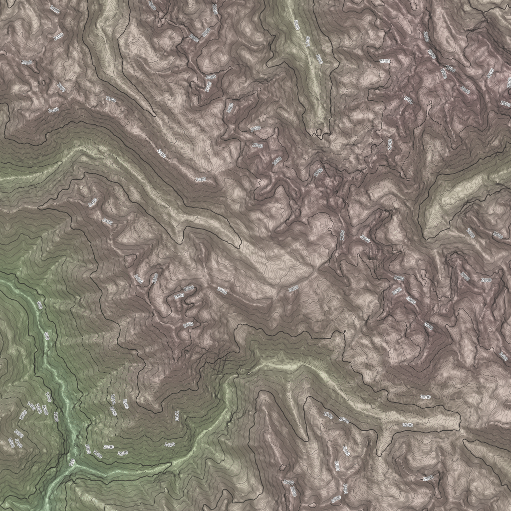
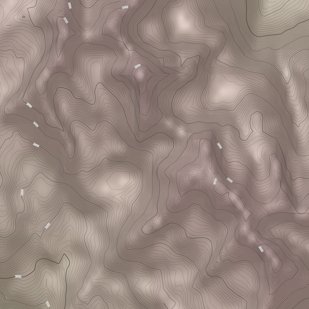
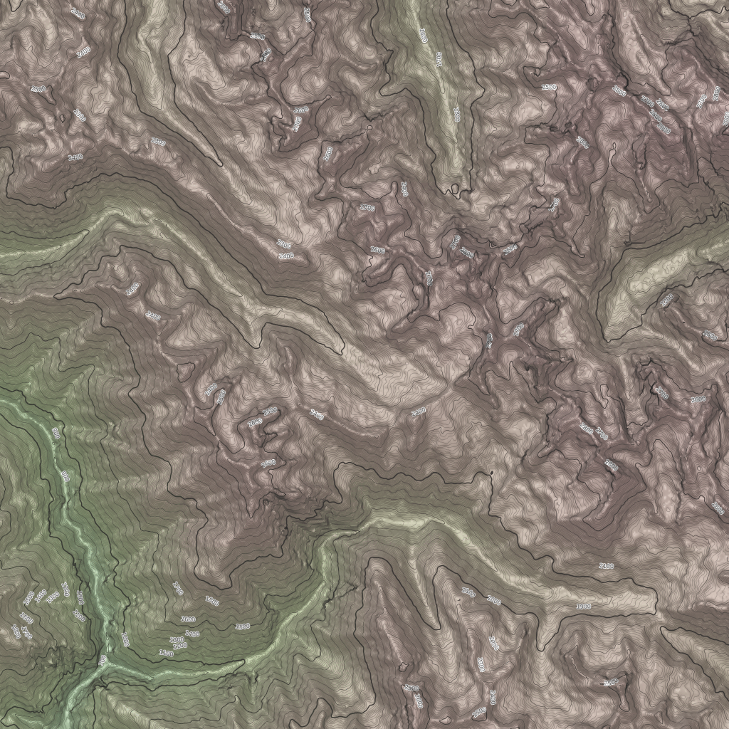
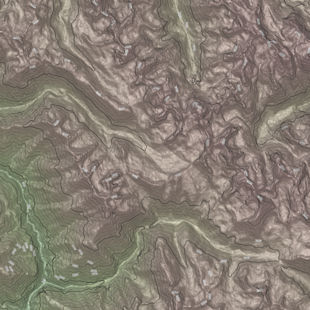
This time you'll probably notice a difference: there's this new contours table with a couple of indexes. This table contains data that I'll be using for drawing hypsometric lines (also know as contour lines) in my map. This 21GiB table contains all the data from 0 to 4000+m in 50m increments for the whole Europe and some parts of Africa and Asia, except for that above 60°, which means that Iceland, most of Scandinavia and the North of Russia is out. At that size, I think it's a bargain.

As with jburgess' data, we have the intermediate data, and quite a lot. Besides the 21GiB extra for contours, we have notably 42+52+2+7GiB for ways. In practice this means that, besides of some of my files, OSM+contour data uses almost all the 220GiB of SSD space, so I'll just move all my stuff out of the SSD :( Another alternative would be to just reimport the whole data from time to time (once a month or each time I update my rendering rules, which I plan to do based on openstreetmap-carto's releases, but not on each one of them).

During the import I logged the memory usage of the 10 more memory hungry processes in the machine with this command:

( while true; do date -R; ps ax -o rss,vsize,pid,cmd | sort -rn | head; sleep 60; done ) | tee -a mem.log

Then I massaged that file with a little bit of Python and obtained a CVS file which I graphed with LibreOffice. I tried several formats and styles, but to make things readable I only graphed the sum of all the postgres processes and osm2psql. This is the final graph:

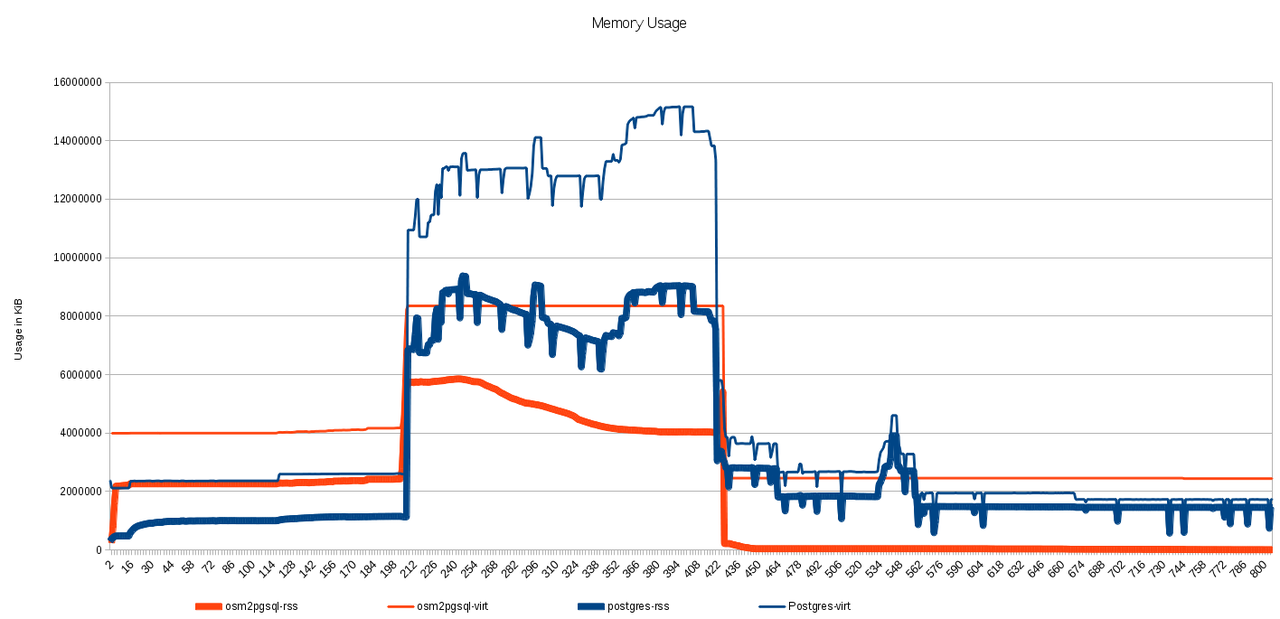
Here you can see 4 lines, 2 for the sum of postgres and two for osm2psql. The thick lines graph the RSS for them, which is the resident, real RAM usage of that process. The correspondent thin line shows the VIRT size, which is the amount of memory malloc()'ed by the processes. As with any memory analysis under Linux, we have the problem that all the processes report also the memory used by the libraries used by them, and if there are common libraries among them, they will be reported several times. Still, for the amounts of memory we're talking about here, we can say it's negligible against the memory used by the data.

In the graph we can clearly see the three phases of the import: first filling up the intermediate tables, then the real data tables themselves, then the indexing. The weird curve we can see in the middle phase for osm2psql can be due to unused memory being swapped out. Unluckily I didn't log the memory/swap usage to support this theory, so I'll have it in account for the next run, if there is one. In any case, the peak at the end of the second phase seems to also support the idea.

One thing that surprises me is the real amount of memory used by osm2psql. I told him to use 2GiB for cache, but at its peak, it uses 3 times that amount, and all the time it has another 2GiB requested to the kernel. The middle phase is also hard on postgres, but it doesn't take that much during indexing; luckily, at that moment osm2psql has released everything, so most of the RAM is used as kernel cache.

13 paragraphs later, I finally write about the reason of this post, updating the database with daily diffs. As I already mentioned, the data as imported almost took all the space available, so I was very sensitive about the amount of space used by them. But first to the sizes and times.

The file 362.osc.gz, provided by Geofabrik as the diff for Europe for Mar05 weights almost 25MiB, but it's compressed XML inside. Luckily osm2psql can read them directly. Here's the summary of the update:

$ osm2pgsql --append --database gis --slim --flat-nodes /home/mdione/src/projects/osm/nodes.cache --cache 2048 --number-processes 4 --unlogged --bbox -11.9531,34.6694,29.8828,58.8819 362.osc.gz
Node-cache: cache=2048MB, maxblocks=262145*8192, allocation method=11
Mid: loading persistent node cache from /home/mdione/src/projects/osm/nodes.cache
Maximum node in persistent node cache: 2701131775
Mid: pgsql, scale=100 cache=2048

Reading in file: 362.osc.gz
Processing: Node(882k 3.7k/s) Way(156k 0.65k/s) Relation(5252 25.50/s)  parse time: 688s [11m28]

Node stats: total(882823), max(2701909278) in 240s [4m00]
Way stats: total(156832), max(264525413) in 242s [4m02]
Relation stats: total(5252), max(3554649) in 206s [3m26]

Going over pending ways...
Maximum node in persistent node cache: 2701910015
        122396 ways are pending

Using 4 helper-processes
Process 3 finished processing 30599 ways in 305 sec [5m05]
Process 2 finished processing 30599 ways in 305 sec
Process 1 finished processing 30599 ways in 305 sec
Process 0 finished processing 30599 ways in 305 sec
122396 Pending ways took 307s at a rate of 398.68/s [5m07]

Going over pending relations...
Maximum node in persistent node cache: 2701910015
        9432 relations are pending

Using 4 helper-processes
Process 3 finished processing 2358 relations in 795 sec [13m15]
Process 0 finished processing 2358 relations in 795 sec
Process 1 finished processing 2358 relations in 795 sec
Process 2 finished processing 2358 relations in 810 sec [13m30]
9432 Pending relations took 810s at a rate of 11.64/s

node cache: stored: 675450(100.00%), storage efficiency: 61.42% (dense blocks: 494, sparse nodes: 296964), hit rate: 5.12%

Osm2pgsql took 1805s overall [30m05]

This time is in the order of minutes instead of hours, but still, ~30m for only 25MiB seems a little bit too much. If I process the diff files daily, it would take ~15h a month to do it, but spread in ~30m stretches on each day. Also, that particular file was one of the smallest I have (between Mar03 and Mar17); most of the rest are above 30MiB, up to 38MiB for Mar15 and 17 each. Given the space problems that this causes, I might as well import before each rerender. Another thing to note is that the cache is quite useless, falling from ~20% to ~5% hit rate. I could try with lower caches too. The processing speeds are awfully smaller than at import time, but the small amount of data is the prevailing here.

Sizes:

 Schema |        Name        |   Type   | Owner  |    Size    | Description
--------+--------------------+----------+--------+------------+-------------
 public | contours           | table    | mdione | 21 GB      |
 public | contours_gid_seq   | sequence | mdione | 8192 bytes |
 public | geography_columns  | view     | mdione | 0 bytes    |
 public | geometry_columns   | view     | mdione | 0 bytes    |
 public | planet_osm_line    | table    | mdione | 11 GB      |
 public | planet_osm_nodes   | table    | mdione | 16 kB      |
 public | planet_osm_point   | table    | mdione | 2184 MB    |
 public | planet_osm_polygon | table    | mdione | 23 GB      |
 public | planet_osm_rels    | table    | mdione | 892 MB     |
 public | planet_osm_roads   | table    | mdione | 2174 MB    |
 public | planet_osm_ways    | table    | mdione | 42 GB      |
 public | raster_columns     | view     | mdione | 0 bytes    |
 public | raster_overviews   | view     | mdione | 0 bytes    |
 public | spatial_ref_sys    | table    | mdione | 3224 kB    |

 Schema |           Name           | Type  | Owner  |       Table        |  Size   | Description
--------+--------------------------+-------+--------+--------------------+---------+-------------
 public | contours_height          | index | mdione | contours           | 268 MB  |
 public | contours_pkey            | index | mdione | contours           | 268 MB  |
 public | contours_way_gist        | index | mdione | contours           | 1144 MB |
 public | planet_osm_line_index    | index | mdione | planet_osm_line    | 4024 MB |
 public | planet_osm_line_pkey     | index | mdione | planet_osm_line    | 756 MB  |
 public | planet_osm_nodes_pkey    | index | mdione | planet_osm_nodes   | 16 kB   |
 public | planet_osm_point_index   | index | mdione | planet_osm_point   | 1494 MB |
 public | planet_osm_point_pkey    | index | mdione | planet_osm_point   | 566 MB  |
 public | planet_osm_polygon_index | index | mdione | planet_osm_polygon | 8210 MB |
 public | planet_osm_polygon_pkey  | index | mdione | planet_osm_polygon | 1955 MB |
 public | planet_osm_rels_idx      | index | mdione | planet_osm_rels    | 352 kB  |
 public | planet_osm_rels_parts    | index | mdione | planet_osm_rels    | 676 MB  |
 public | planet_osm_rels_pkey     | index | mdione | planet_osm_rels    | 38 MB   |
 public | planet_osm_roads_index   | index | mdione | planet_osm_roads   | 358 MB  |
 public | planet_osm_roads_pkey    | index | mdione | planet_osm_roads   | 78 MB   |
 public | planet_osm_ways_idx      | index | mdione | planet_osm_ways    | 2165 MB |
 public | planet_osm_ways_nodes    | index | mdione | planet_osm_ways    | 52 GB   |
 public | planet_osm_ways_pkey     | index | mdione | planet_osm_ways    | 6926 MB |
 public | spatial_ref_sys_pkey     | index | mdione | spatial_ref_sys    | 104 kB  |

3MiB more of points, 21+5+1MiB more of rels, 45+1MiB more of roads, 0+2+8MiB more of lines, 0+3MiB for polygons, 0+4+4MiB for ways. In total, some 97MiB more. I tried a VACUUM at the end, but no space was gained, and I don't have enough space for VACUUM FULL. As VACUUM does not defragment, a second and third updates should make use of the internal fragmentation. Let's see.

363.osc.gz is the smalest file I have, at ~22MiB. The times are internally different, but overall looks proportional:

$ osm2pgsql --append --database gis --slim --flat-nodes /home/mdione/src/projects/osm/nodes.cache --cache 2048 --number-processes 4 --bbox -11.9531,34.6694,29.8828,58.8819 363.osc.gz
Maximum node in persistent node cache: 2701910015

Reading in file: 363.osc.gz
Processing: Node(750k 3.3k/s) Way(128k 0.44k/s) Relation(4264 15.73/s)  parse time: 792s

Node stats: total(750191), max(2703147051) in 230s
Way stats: total(128987), max(264655143) in 291s
Relation stats: total(4264), max(3556985) in 271s

Going over pending ways...
Maximum node in persistent node cache: 2703148031
        94490 ways are pending

Using 4 helper-processes
Process 0 finished processing 23623 ways in 238 sec
Process 2 finished processing 23622 ways in 238 sec
Process 1 finished processing 23623 ways in 238 sec
Process 3 finished processing 23622 ways in 239 sec
94490 Pending ways took 241s at a rate of 392.07/s

Going over pending relations...
Maximum node in persistent node cache: 2703148031
        8413 relations are pending

Using 4 helper-processes
Process 1 finished processing 2103 relations in 443 sec
Process 3 finished processing 2103 relations in 445 sec
Process 0 finished processing 2104 relations in 450 sec
Process 2 finished processing 2103 relations in 452 sec
8413 Pending relations took 453s at a rate of 18.57/s

node cache: stored: 576093(100.00%), storage efficiency: 60.50% (dense blocks: 437, sparse nodes: 252366), hit rate: 5.07%

Osm2pgsql took 1488s overall

The table sizes keep growing, as expected: OSM data does nothing but grow; my free space does nothing but shrink, currently at mere 249MiB. Given that the intermediate tables are dropped at the end of the second import phase, it only makes sense to do full imports from time to time, before updating the rendering rules. Munitely is not for me.

Since I started playing with rendering maps I included some kind of elevation info for highlighting mountains. At the beginning it was just hillshading provided by some german guy (I don't have the reference on me right now), but after reading Tilemill's terrain data guide, I started using DEMs to generate 4 different layers: elevation coloring, slope shading, hillshading and contour lines.

When I started I could find only three DEM sources: SRTM 3arc and ViewFinderPanoramas (1arc and 3arc). The second one tries to flatten plains (for instance, the Po's plain nearby to where I live), where it generates some ugly looking terracing. The third one, when I downloaded the corresponding tile (they're supposed to be 1x1 degrees), its medatada reported an extension between 7 and 48 degrees east, and between 36 and 54 degrees north, and that its size is 147602x64801 pixels. I also remember stitching all the tiles covering Europe, just to get a nice 1x1 degrees hole in the North Adriatic sea. Not having much time to pre or post process the data, I decided to stick to SRTM.

Things changed at the end of last year. The US government decided to release 1arc, 30m global coverage (previously that resolution covered only the US). I started playing with the data mid January, only to find that it is not void-filled: this DEMs are derived from the homonymous Shuttle mission, which used radar to get the data. Radar gets very confused when water is involved; this is no problem on rivers, lakes or sea, where elevation is constant relative to the coast, but it's a problem on snow covered mountains, glaciers and even clouds. This means that the data has NODATA holes. The SRTM 3arc v4.1 I was using had these 'voids' filled; deFerrantis has painstakingly been filling these voids too by hand, using topographic maps as reference.

So I set up to fill these voids too. But first let's see how the original data looks like. All the images are for the area near Isola 2000, a ski station I go often. The first image is how this looks on the SRTM 3arc v4.1:

This is a 4x4 grid of 256x256 pixel tiles (1024x1024 in total) at zoom level 13. The heights range from ~700m up to ~2600m, and the image combines all the 4 layers. It already starts showing some roundness in the terrain, specially in ridges and mountain tops; even at the bottom of the deep valleys.

For contrast, this is deFerrantis data:

This is the first time I really take a look on the result; it doesn't seem to be much better that 3arc. Here's the terracing I mentioned:

For contrast, check what 1arc means:

From my point of view, the quality is definitely better. Peaks, crests and valleys are quite sharp. As for the mountain sides, they look rugged. My appreciation is this reflects better the nature of the terrain in question, but Christoph Hormann of Imagico.de views it as sample noise. He has worked a lot on DEMs to generate very beautiful maps.

But then we have those nice blue lagoons courtesy of voids (the blue we can see is the water color I use in my maps). So, how to proceed?

The simplest way to fix this is covering the voids with averages calculated from the data at the seams of the voids. GDAL has a tool for that called, of course, gdal_fillnodata.py. This is the outcome:

At first this looks quite good, but once we start to zoom in (remember there are at least 5 more zoom levels), we start to see some regular patterns:

Another option is to use deFerrantis' data to fill the voids. For this we need to merge both datasets. One way to do it is using GDAL's gdalwarp tool. We create a file piling up layers of data; first the most complete one, then the layers with holes:

gdalwarp deFerrantis/N44E007.hgt mixed.tif
gdalwarp SRTM_1arc_v3/n44_e007_1arc_v3.tif mixed.tif

This looks like this:

I have to be honest, it doesn't look good. Both files declare the same extents and resolution (their metadata is similar, but the second file has more), but if you compare the renders for SRTM_1arc_v3 and deFerrantis, you will notice that they don't seem to align properly.

The last simple option would be to upsample SRTM_3arc_v4.1 and then merge like before, but it took me a while to figure out the right parameters:

gdalwarp -te 6.9998611 43.9998611 8.0001389 45.0001389 -tr 0.000277777777778 -0.000277777777778 -rb SRTM_3as_v4.1/srtm_38_04.tif srtm_1as_v3-3as_v4.1.tif
Creating output file that is 3601P x 3601L.
Processing input file SRTM_3as_v4.1/srtm_38_04.tif.
Using internal nodata values (eg. -32768) for image SRTM_3as_v4.1/srtm_38_04.tif.
0...10...20...30...40...50...60...70...80...90...100 - done.
gdalwarp SRTM_1as_v3/n44_e007_1arc_v3.tif srtm_1as_v3-3as_v4.1.tif
Processing input file SRTM_1as_v3/n44_e007_1arc_v3.tif.
Using internal nodata values (eg. -32767) for image SRTM_1as_v3/n44_e007_1arc_v3.tif.
0...10...20...30...40...50...60...70...80...90...100 - done.

The complex part was the -te and -tr parameters. The 3 arc file covers a 5x5 degrees zone at 40-45°N, 5-10°E. The 1 arc file only covers 44-45°N, 7-8°E, so I need to cut it out. I use the -te option for that, but according the doc it's «[to] set georeferenced extents of [the] output file to be created». This means the degrees of the W, S, E and N limits of the output file. Note that the actual parameters are 1.5" off those limits; I took those limits from the original 1 arc file.

The second one is even more cryptic: «[to] set [the] output file resolution (in target georeferenced units)». This last word is the key, units. According to gdalinfo, both files have a certain pixel size in units declared in the projection. Both declare UNIT["degree",0.0174532925199433]; “degree“ has a clear meaning; the float besides it is the size of the unit in radians (π/180). So the parameters for -tr is how many units (degrees) does a pixel represent (or, more accurately, how many degrees are between a pixel center and the next one). Notice that the vertical value is negative; that's because raster images go from North to South, but degrees go the other way around (North and East degrees are positive, South and West negative). In any case, I also just copied the pixel size declared in the 1 arc file.

After all this dissertation about GeoTIFF metadata, finally the resulting DEM:

As I said earlier, I don't have much time to invest in this; my map is mostly for personal consumption and I can't put much time on it. so my conclusion is this: if I can manage the 9x data size, I think I'm going this way.

A short note. As both the signal module doc and the subprocess module doc (almost at the end, when it finally goes around to talk about the restore_signals parameter), Python3 disables the following signals, so it can properly report them as exceptions:

• SIGPIPE
• SIGXFZ
• SIGXFSZ
• SIGINT

But if you're executing processes with any of the os.exec*() functions, you have to restore them by hand. Of course, the option is to use subprocess, which is best for most cases; not for ayrton.

I spent a long time analyzing the process-which-didn't-die-on-SIGPIPE's source code and wondering what was all this about. The I compared the same pipeline under bash and ayrton with strace to find the real culprit.

At work we have Windows workstations, but we develop for Linux (don't ask; in my previous mission in another MegaCorp we had a similar setup for admining Linux servers...). We have access to devel machines via ssh and Samba, but the setup is laughable. I won't go too much into details because it's embarrassing and because I signed some kind of NDA somewhere.

Thing is, I setup a VM with VirtualBox in my workstation, installing a barebones Debian Sid. To have better integration with the Windows host I decided to install the VBox Linux Additions, but for some reason it was not setting up the video side of it. The error message is the one from the title:

Could not find X.org or XFree86 on the guest system. The X Window drivers will not be installed.

Thanks to this post I managed to quickly find out the reason. The step that actually tests and installs the x.org drivers is called like this:

/etc/init.d/vboxadd-x11 setup

If you run it with sh -x you will find out that it actually tests two things: the existence of /usr/lib/xorg/modules, which you can either create or just install the xserver-xorg-video-vesa package, and it tries to run X, which you will find in the xserver-xorg package.

So, TL;DR version: Just install these two packages:

sudo apt-get install xserver-xorg-video-vesa xserver-xorg

Now all works.

One of the most cited ways to accelerate rendering maps with Mapnik is metatiling. This technique is simple: instead of rendering each individual 256x256 PNG file that normally backs a slippy map, render NxN times that (normally with N=8) and split afterwards. mapnik-stylesheet's generate_tiles.py was not capable of doing it, but I hacked a little bit and got it to do it, so after integrating openstreetmap-carto v2.14.1 and fixing some local bugs, I gave it another spin.

This time I also imported the whole Europe data, and expanded the terrain to cover anything above 60°N, taking the height files form De Ferranti's viewfinderpanoramas. This meant that whatever rendering times I got this time, they are not completely comparable to what I obtained before because it's simply handling way more data, specially relative to the terrain data.

So, first, a short revisit to importing. Here's the summary:

mdione@diablo:/var/lib/data/mdione/src/projects/osm/data/osm$ osm2pgsql \
    --create --drop --database gis --slim --flat-nodes /home/mdione/src/projects/osm/nodes.cache \
    --cache 2048 --number-processes 4 --unlogged europe-latest.osm.pbf
osm2pgsql SVN version 0.82.0 (64bit id space)

Node-cache: cache=2048MB, maxblocks=262145*8192, allocation method=11
Mid: loading persistent node cache from /home/mdione/src/projects/osm/nodes.cache
Allocated space for persistent node cache file
Maximum node in persistent node cache: 0
Mid: pgsql, scale=100 cache=2048

Reading in file: europe-latest.osm.pbf
Processing: Node(1225816k 799.6k/s) Way(151242k 17.71k/s) Relation(1872470 338.91/s)  parse time: 15596s [4h20m]
Node stats: total(1225816996), max(2884224404) in 1533s [0h26m]
Way stats: total(151242682), max(284701738) in 8538s [2h22m]
Relation stats: total(1872475), max(3776697) in 5525s [1h32m]

Going over pending ways...
Maximum node in persistent node cache: 2884632575
        110980610 ways are pending
Using 4 helper-processes [but only 1 is used, the others failed, dunno why]
Mid: loading persistent node cache from /home/mdione/src/projects/osm/nodes.cache
Maximum node in persistent node cache: 2884632575
Process 0 finished processing 110980610 ways in 34202 sec [9h30m]
110980610 Pending ways took 34202s at a rate of 3244.86/s

Going over pending relations...
Maximum node in persistent node cache: 2884632575
        0 relations are pending
Using 4 helper-processes
Process 2 finished processing 0 relations in 2 sec
Process 3 finished processing 0 relations in 2 sec
Process 0 finished processing 0 relations in 3 sec
Process 1 finished processing 0 relations in 3 sec
0 Pending relations took 3s at a rate of 0.00/s

node cache: stored: 203128264(16.57%), storage efficiency: 75.67% (dense blocks: 138131, sparse nodes: 63494657), hit rate: 17.62%

Stopped table: planet_osm_rels in 1s
Stopped table: planet_osm_nodes in 1s
Stopped table: planet_osm_ways in 3s

All indexes on  planet_osm_roads created  in 4679s [1h18m]
All indexes on  planet_osm_point created  in 6093s [1h41m]
All indexes on  planet_osm_line created  in 9703s [2h42m]
All indexes on  planet_osm_polygon created  in 12735s [3h32m]

Osm2pgsql took 62780s overall [17h26m]

Only ~3h30m more than importing a part of Europe, I think it's manageable. I still don't know what to make out of the cache/storage efficiency line, but it's clearly related to the small size of the cache.

About the rendering, I only rendered up to zoom level 11, as I discussed before, but that limit was mostly due to the fact that going all the way down to 14 took too much time. But after viewing how much less rendering took this time, I most probably revert that change. Take a look at the graph:

This graph shows the average and total time for rendering up to zoom level 11 with single tiling (actually it's the old data I showed previously) and metatiling 8x8. The total time uses the logarithmic scale on the right. The average in the second case is the division between the total time and the amount of final individual tiles, which are produced by cutting the metatile in as many single tiles as the minimum between 2^z and 64, so zoom levels 0-2 don't produce spurious images. The times are amazing. Notice that from time to time the total time took more in the metatile version than in the single tile version, but the are two factors that impact here. One is that due to metatiling, I'm rendering tiles that with single tiling I wouldn't due to the fact that now I can only cut in increments of 8 instead of one. Two, now I'm rendering the whole Europe instead of just a big part of it. This makes the amount of tiles produced to be between 6 to 10 times more.

Still, take a look at the average rendering times for metatiling, and specially at the last column in the table, which is not graphed: it's the proportion between the average tile rendering time, meta to single. It's mostly below the 10%, except for a couple of zoom levels that either produce few tiles (ZL 2, 16 tiles) or stay under 15% (ZL 4). This is ridiculously low, which means fast. I will first finish rendering my zone down to ZL 18 and then render the rest down to ZL 14 to have more complete, comparable graphs.

I've been advancing a lot with ayrton. A lot of things already work and I'm still toying with the final syntax, but this is not what I came to talk about.

Since its inception, I had one particular idea for a scripting language: the ability to connect through ssh to another machine and execute some code there, without a requirement that the code must be already a script in the remote machine, and that has sane ways to reference variables both local to the instance of the code running in the remote machine and variables local to the 'parent' script. This is more or less what I'm talking about:

ssh $user_machine '\
    cd /foo; \
    cd $(find . -type d -name "Fo-Obarbaz-*" | sort -u | tail -1); \
    file=$(ls -1 *_LOG); \
    echo "File: $file"; \
    cat $file' > local_file

This example is simple in the sense that it only references variable local to the remote execution; just try to imagine how much escaping you would need for referencing both types of variables.

Python3 has a very handy construct for this: context managers. Imagine that you could write:

with ssh (user_machine, _out=open (local_file, 'w+')):
    cd ('/foo')
    cd (tail (sort (find ('. -type d -name Fo-Obarbaz-*'), '-u') '-1'))
    file= ls ('-l', bash ('*_LOG'))
    print ("File: %s" % file)
    cat (file)

That's my current goal. So I set off to find how to achieve this. The first part of the journey is to find the body of the with statement. Suppose this simpler code:

# file with_ssh.ay
with ssh ('localhost'):
    print ('yes!')

Enter the ast module:

import ast

t= ast.parse (open ('with_ssh.ay').read ())
for node in ast.walk (t):
    if type (node)==ast.With and node.items[0].context_expr.func.id=='ssh':
        code= node.body

f= ast.Module(body=code)
f_c= compile (f, 'foo', 'exec')
exec (f_c)

This small piece of code prints yes! without a hitch. My work is done here...

... except that I still have to find how to send the code via ssh¹, most probably with all its dependencies, probably check that the python version matches, compile it and execute it there. And chose a way to reference variables in the calling environment and/or transmit them. But that's for another post :)

This kind of AST manipulation could also allow me to properly implement |.

Last night I got an idea: start implementing some stuff on top of Elevation. The first thing I thought of was the ability to save markers in cookies, and to recover them every time the map was accessed. This would allow anybody to safely add personal markers on top of it without having to trust me (except for the map service). This might lead to something else entirely later, but for now that was the goal.

So the first step was to find out how to access cookies in js. It seems that there is no native way to do it, and you have to parse them for yourself from the document.cookie attribute. Luckily someone already wrote some code for it. There was no license, but I think it's ok. Then I added another function to have a list of all the cookies whose name starts with some prefix, based on the readCookie() function:

function readCookies(prefix) {
    var nameEQ = prefix + '_';
    var ca = document.cookie.split(';');
    var ans = [];
    j= 0;
    for (var i = 0; i < ca.length; i++) {
        var index = 0;
        var c = ca[i];
        while (c.charAt(index) == ' ') {
            index = index + 1;
        }
        if (c.indexOf(nameEQ) == index) {
            // keep reading, find the =
            while (c.charAt(index) != '=') {
                index = index + 1;
            }
            ans[j] = c.substring(index + 1, c.length);
            j= j+1;
        }
    }
    return ans;
}

The next step was to encode and decode markers into strings. The format I decided is simple: CSV, lat,lon,text,URL. So, here's the function that converts cookies to markers:

function markersFromCookies () {
    var cookies= readCookies ("marker");

    for (var i= 0; i<cookies.length; i++) {
        var cookie= cookies[i];

        var data= cookie.split (',');
        // it's lat,lon,text,url
        var marker= L.marker([data[0], data[1]]).addTo (map);
        // TODO: reconstruct the url in case it got split
        if (data[3].length>0) {
            marker.bindPopup ('<a href="'+data[3]+'">'+data[2]+'</a>').openPopup ();
        } else {
            marker.bindPopup (data[2]).openPopup ();
        }
    }
}

20 lines of code and there already is a TODO comment :) That's because URLs can have commas in them, but for the moment I'm thinking in short URLs from sites like bitly.

All this was working perfectly in Firefox' scratchpad. Then I decided to put it in "production". For that I took all the js from the original page and put it in a file, along with all these functions, I removed the permanent marker from my map, converting it into a cookie, pushed the code, reloaded and... it broke.

This is not the first time I see js fall apart. Last year I helped PyCon.ar's organization with the site, specifically the map showing the city with markers for the venue and the bus station. I even had to map the venue because it was not in OSM's data :) If you follow that link, you'll see that the popups are completely broken. These things were working perfectly in vacuum, but when I integrated it into the page it just fell apart. I never found out why.

In my current situation, if I try to run markersFromCookies() in scratchpad, this is what I get:

Exception: t.addLayer is not a function
o.Marker<.addTo@http://cdn.leafletjs.com/leaflet-0.7.2/leaflet.js:7
markersFromCookies@http://grulicueva.homenet.org/~mdione/Elevation/local.js:59
@Scratchpad/1:1

Basically, that's the call to L.marker().addTo(). Maybe the constructor is not working anymore, maybe something else entirely. At least this time a dim light in the back of my head told me maybe the map variable is not global as it seems to be from scratchpad, so I simply passed the map from setup_map() to markersFromCookies() and now it works. Notice that the error message never mentioned this fact but something else entirely. I'm just glad I didn't have to follow the hint and debug Leaflet's to find out this. All I hope now is that I don't go insane with this small project.

Next steps: adding new markers and sharing!