Finding data peaks with grafana and prometheus

While doing my research for the OSM import and update posts I used one of the simplest graphs I have in my Grafana instance: disk usage. Because the source is Prometheus' node_exporter's node_filesystem_* series, I have to use an expression:

node_filesystem_size_bytes - node_filesystem_free_bytes

In the same graph I also have just node_filesystem_size_bytes drawn as a dotted line to see what's the limit of each disk (this system has only two for the moment). But for the investigation itself I also wanted to know the peak of the data usage, and in particular when it happened. So my train of thought was this:

“I just need to take the max() of the data.”

Wrong. max() is an aggregator operator (yes, not a function; I thought it was one, as many examples use parenthesis) and does not do what I want. If you graph that, you only get the same line as the max of all the graphed series, which, in retrospective, makes sense.

So I try around more stuff and I can't get it done. As in many other cases, I head over to #prometheus@libera.chat for answers. The first part of the solution is max_over_time(), which is a function (yes this time) that takes a range vector and produces an instant vector. Now, I want to see the max over the graphed range, which will change as I zoom in and out in Grafana looking at different parts of the process, not the max over the whole series or some other fixed number, so I'll be using Grafana's $__range variable. So this must be it:

max_over_time((node_filesystem_size_bytes - node_filesystem_free_bytes)[$__range])

Right?

Wrong, again. parse error: ranges only allowed for vector selectors.

sigh

I cheated again and got the answer from the IRC channel. The answer is subqueries:

max_over_time((node_filesystem_size_bytes - node_filesystem_free_bytes)[$__range:])

Spot the difference, I challenge you.

Let's take a step back.

To start with, I realized something that is quite subtle here. If you read the documentation closely, it talks not only about instant and range vectors, but also about instant and range vector selectors. In my head, as a programmer, I now have to think of them in terms of foo being a IVS that 'returns' and IV; if you add a range, as in foo[1m], you get a RVS that 'returns' an RV1.

Then, as this video mentions, binary operators return mostly IVs, and that's why you can't apply a range to them, because they're not selectors, but final values.

But.

The subquery syntax2, among other things, allows you to 'apply a range' to your IV and get a RV. One slight difference is that on a RVS you might get different amount of data point across series, while with a subquery, I think, the IVS in the subquery is evaluated for every period, so you always get a value for each time. I don't have an example without data, but if you run a subquery, you'll see all the timestamps don't have a decimal digits (they're integers) because they align with the scrapping period (15s):

node_filesystem_free_bytes[1m]
------------------------------
node_filesystem_free_bytes{device="/dev/sda2",fstype="ext4",instance="127.0.0.1:9100",job="node",mountpoint="/"}
    217540681728 @1692981943.193
    217540648960 @1692981958.194
    217540624384 @1692981973.193
    217540595712 @1692981988.193
[...]

vs

node_filesystem_free_bytes[1m:]
-------------------------------
node_filesystem_free_bytes{device="/dev/sda2",fstype="ext4",instance="127.0.0.1:9100",job="node",mountpoint="/"}
    217540513792 @1692982035
    217540476928 @1692982050
    217540448256 @1692982065
    217540423680 @1692982080
[...]

Again, spot the difference. Go ahead.

So for now part of the solution feels like a black box. I hope one day understand all this, but for now this will have to be enough.

But I haven't finished.

That query only gives you an instant vector. If you graph that, you also get a line following the original data! The tricks are:

  • Tell Grafana to do an 'instant query'.

This makes Grafana get a single value, not a value per graph period.

  • Tell Grafana to extend the graph by using a series override and apply "Transform: Constant".

This makes that single dot per series a line.

The final graph:

You can see the import peaks at the left. Disk capacity is drawn with thick dashes. The other disk's usage didn't change in all that time, so there's no peak and the max line follows the graph.


  1. At the beginning I thought the problem was that expression values were not instant vectors. They seemed to be something else, and you that couldn't range them. The alternative is to create a recording rule, which is a calculated (from an expression) data series, from which you can get ranges because you can use an IVS to reference them. 

  2. Good luck trying to get something useful from that. Try this one instead. 

Disk usage while updating an OSM rendering database

Now the new part. I have never updated an OSM rendering table, so let's see what the docs say about it:

To keep an osm2pgsql database up to date you have two options: you either provide the original import data file, or you provide the replication URL. In my case, the latter is http://download.geofabrik.de/europe-updates/, but as you can see, it can be inferred from the extract; it even picks up the right date1:

$ osm2pgsql-replication init --verbose --port 5433 --database gis --osm-file europe-latest.osm.pbf
2023-08-23 15:07:18 [DEBUG]: Replication information found in OSM file header.
2023-08-23 15:07:18 [DEBUG]: Replication URL: http://download.geofabrik.de/europe-updates
2023-08-23 15:07:18 [DEBUG]: Replication sequence: 3787
2023-08-23 15:07:18 [DEBUG]: Replication timestamp: 2023-08-11T20:21:59Z
2023-08-23 15:07:18 [INFO]: Initialised updates for service 'http://download.geofabrik.de/europe-updates'.
2023-08-23 15:07:18 [INFO]: Starting at sequence 3787 (2023-08-11 20:21:59+00:00).

Then the update is really simple: you just tell it to do it and it will do it, automatically! The only condition is that you give the update the same parameters you gave to the original osm2pgsql invocation. It will proceed to download a batch of updates until some value is reached (around 120MiB?), then call osm2pgsql, rinse, repeat, until all missing updates have been applied:

$ osm2pgsql-replication update --verbose --port 5433 --database gis -- --cache 0 --number-processes 4 --slim --flat-nodes $(pwd)/nodes.cache --hstore --multi-geometry --style $osm_carto/openstreetmap-carto.style --tag-transform-script $osm_carto/openstreetmap-carto.lua
2023-08-23 15:13:16 [INFO]: Using replication service 'http://download.geofabrik.de/europe-updates'. Current sequence 3787 (2023-08-11 22:21:59+02:00).
2023-08-23 15:13:16 [DEBUG]: Starting new HTTP connection (1): download.geofabrik.de:80
2023-08-23 15:13:16 [DEBUG]: http://download.geofabrik.de:80 "GET /europe-updates/state.txt HTTP/1.1" 200 123
2023-08-23 15:13:16 [DEBUG]: Calling osm2pgsql with: /usr/bin/osm2pgsql --append --slim --prefix planet_osm --cache 0 --number-processes 4 --slim --flat-nodes /home/mdione/src/projects/osm/data/osm/nodes.cache --hstore --multi-geometry --style /home/mdione/src/projects/osm/osm-carto/openstreetmap-carto.style --tag-transform-script /home/mdione/src/projects/osm/osm-carto/openstreetmap-carto.lua -d gis -P 5433 /tmp/tmpk7ml1gi9/osm2pgsql_diff.osc.gz
2023-08-23 15:13:16 [DEBUG]: Importing from sequence 3787
2023-08-23 15:13:16 [DEBUG]: Starting new HTTP connection (1): download.geofabrik.de:80
2023-08-23 15:13:16 [DEBUG]: http://download.geofabrik.de:80 "GET /europe-updates/state.txt HTTP/1.1" 200 123
2023-08-23 15:13:16 [DEBUG]: Starting new HTTP connection (1): download.geofabrik.de:80
2023-08-23 15:13:16 [DEBUG]: http://download.geofabrik.de:80 "GET /europe-updates/000/003/788.osc.gz HTTP/1.1" 200 30348254
2023-08-23 15:13:25 [DEBUG]: Downloaded change 3788. (389531 kB available in download buffer)
2023-08-23 15:13:25 [DEBUG]: Starting new HTTP connection (1): download.geofabrik.de:80
2023-08-23 15:13:25 [DEBUG]: http://download.geofabrik.de:80 "GET /europe-updates/000/003/789.osc.gz HTTP/1.1" 200 35284953
2023-08-23 15:13:36 [DEBUG]: Downloaded change 3789. (245491 kB available in download buffer)
2023-08-23 15:13:36 [DEBUG]: Starting new HTTP connection (1): download.geofabrik.de:80
2023-08-23 15:13:36 [DEBUG]: http://download.geofabrik.de:80 "GET /europe-updates/000/003/790.osc.gz HTTP/1.1" 200 32891529
2023-08-23 15:13:46 [DEBUG]: Downloaded change 3790. (114339 kB available in download buffer)
2023-08-23 15:13:46 [DEBUG]: Starting new HTTP connection (1): download.geofabrik.de:80
2023-08-23 15:13:46 [DEBUG]: http://download.geofabrik.de:80 "GET /europe-updates/000/003/791.osc.gz HTTP/1.1" 200 35347966
2023-08-23 15:13:57 [DEBUG]: Downloaded change 3791. (-26371 kB available in download buffer)
2023-08-23 15:14:16  osm2pgsql version 1.8.0
2023-08-23 15:14:16  Database version: 15.3 (Debian 15.3-0+deb12u1)
2023-08-23 15:14:16  PostGIS version: 3.3
2023-08-23 15:14:16  Setting up table 'planet_osm_point'
2023-08-23 15:14:16  Setting up table 'planet_osm_line'
2023-08-23 15:14:16  Setting up table 'planet_osm_polygon'
2023-08-23 15:14:16  Setting up table 'planet_osm_roads'
2023-08-23 16:26:17  Reading input files done in 4321s (1h 12m 1s).
2023-08-23 16:26:17    Processed 3014131 nodes in 1506s (25m 6s) - 2k/s
2023-08-23 16:26:17    Processed 687625 ways in 977s (16m 17s) - 704/s
2023-08-23 16:26:17    Processed 28176 relations in 1838s (30m 38s) - 15/s
2023-08-23 16:27:11  Going over 217062 pending ways (using 4 threads)
Left to process: 0........
2023-08-23 16:30:04  Processing 217062 pending ways took 173s (2m 53s) at a rate of 1254.69/s
2023-08-23 16:30:04  Going over 89496 pending relations (using 4 threads)
Left to process: 0.......
2023-08-23 17:24:42  Processing 89496 pending relations took 3277s (54m 37s) at a rate of 27.31/s
2023-08-23 17:24:43  Done postprocessing on table 'planet_osm_nodes' in 0s
2023-08-23 17:24:43  Done postprocessing on table 'planet_osm_ways' in 0s
2023-08-23 17:24:43  Done postprocessing on table 'planet_osm_rels' in 0s
2023-08-23 17:24:43  All postprocessing on table 'planet_osm_point' done in 0s.
2023-08-23 17:24:43  All postprocessing on table 'planet_osm_line' done in 0s.
2023-08-23 17:24:43  All postprocessing on table 'planet_osm_polygon' done in 0s.
2023-08-23 17:24:43  All postprocessing on table 'planet_osm_roads' done in 0s.
2023-08-23 17:24:43  osm2pgsql took 7827s (2h 10m 27s) overall.
[...]

I'm not going to put all 4 or 5 iterations, this should be enough. 2h10m to process around 120MiB od data, meaning around 1m/MiB. I have 12 days of updates, each around 30MiB, except for the last three, that are 90, 160 and 130 MiB each, due to an ongoing edit battle. A total of around 620MiB of updates, it's going to take 10h at this pace.

[The next day]

[...]
2023-08-23 23:31:36 [INFO]: Data imported until 2023-08-22 20:21:53+00:00. Backlog remaining: 1 day, 1:09:43.865536

After ~8h10m it finished. Disk space grew 10GiB, which is more than the 10x of the import (more like 15x!). At this pace I should get space issues in around 220 days. On the other hand, these diffs are quite unusual, so probably the stats are skewed. Also, I guess at some point I should redo some of the clustering and analyzing done in the import process, but I don't see anything on the docs, so I'll ask around. There are not big peaks to talk about. The most space I see being freed is around 200MiB.

The osm2pgsql people have automated it to the point where they even provide in their documentation an example systemd unit file to do the updates for you. Check the docs linked above.


  1. Yes, I started writing these posts 13 days ago. 

Disk usage while importing an OSM rendering database

Preface: I wanted to include the updating part in this post, but it got too long already, so I'll split it in two. I will update this post when the second comes out.

TL;DR version: import seems to use a peak of 15x space compared to the .osm.pbf source file, and a final 10x. If you're tight on space, try --number-processes 1, but it will be way slower. You can also save some 4x size if you have 4x RAM (by not using --flat-nodes).

I decided to try and maintain a daily OpenStreetMap rendering database for Europe. The plan is to, at some point, have a rendering server at home, instead of depending of occasional renderings. For this I will use my old laptop, which has a 1TB SSD and only 8GiB of RAM, which I plan to upgrade to 16 at some point. The machines does a few other things (webmail, backups, cloud with only two users, and other stuff), but the usage is really low, so I think it'll be fine.

This week I cleaned up disk space and I prepared the main import. Due to the space constraints I wanted to know how the disk usage evolves during the import. In particular, I wanted to see if there could be a index creation order which could be beneficial for people with limited space for these operations. Let's check the times first2:

$ osm2pgsql --verbose --database gis --cache 0 --number-processes 4 --slim --flat-nodes $(pwd)/nodes.cache --hstore --multi-geometry \
    --style $osm_carto/openstreetmap-carto.style --tag-transform-script $osm_carto/openstreetmap-carto.lua europe-latest.osm.pbf

2023-08-18 15:46:20  osm2pgsql version 1.8.0
2023-08-18 15:46:20  [0] Database version: 15.3 (Debian 15.3-0+deb12u1)
2023-08-18 15:46:20  [0] PostGIS version: 3.3
2023-08-18 15:46:20  [0] Setting up table 'planet_osm_nodes'
2023-08-18 15:46:20  [0] Setting up table 'planet_osm_ways'
2023-08-18 15:46:20  [0] Setting up table 'planet_osm_rels'
2023-08-18 15:46:20  [0] Setting up table 'planet_osm_point'
2023-08-18 15:46:20  [0] Setting up table 'planet_osm_line'
2023-08-18 15:46:20  [0] Setting up table 'planet_osm_polygon'
2023-08-18 15:46:20  [0] Setting up table 'planet_osm_roads'

2023-08-19 20:49:52  [0] Reading input files done in 104612s (29h 3m 32s).
2023-08-19 20:49:52  [0]   Processed 3212638859 nodes in 3676s (1h 1m 16s) - 874k/s
2023-08-19 20:49:52  [0]   Processed 390010251 ways in 70030s (19h 27m 10s) - 6k/s
2023-08-19 20:49:52  [0]   Processed 6848902 relations in 30906s (8h 35m 6s) - 222/s
2023-08-19 20:49:52  [0] Overall memory usage: peak=85815MByte current=85654MByte

Now I wonder why I have --cache 0. Unluckily I didn't leave any comments, so I'll have to check my commits (I automated all this with a script :). Unluckily again, this slipped in in a commit about something else, so any references are lost :( Here are the table sizes1:

        Name        | Type  | Access method |    Size
--------------------+-------+---------------+----------------
 planet_osm_ways    | table | heap          | 95_899_467_776
 planet_osm_polygon | table | heap          | 92_916_039_680 *
 planet_osm_line    | table | heap          | 43_485_192_192 *
 planet_osm_point   | table | heap          | 16_451_903_488 *
 planet_osm_roads   | table | heap          |  6_196_699_136 *
 planet_osm_rels    | table | heap          |  3_488_505_856
 spatial_ref_sys    | table | heap          |      7_102_464
 geography_columns  | view  |               |              0
 geometry_columns   | view  |               |              0

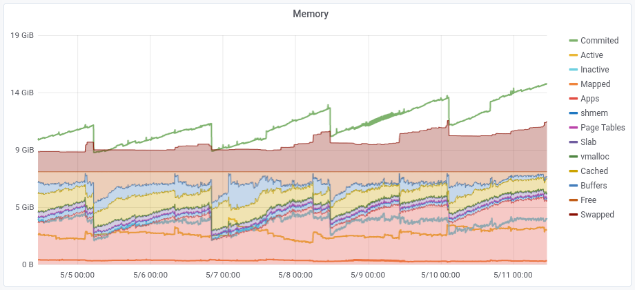
Those marked with * are used for rendering, the rest are kept for update purposes. Let's see the disk usage [click to get the full image]:

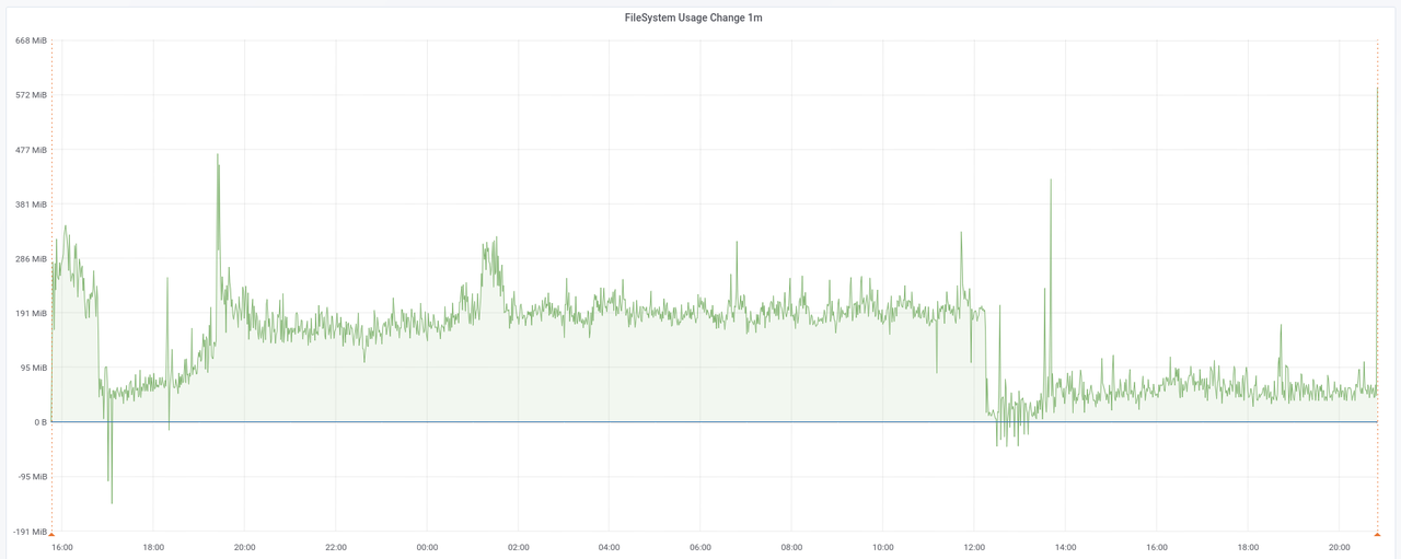
The graph shows the rate at which disk is used during the import of data. We can only see some space being freed around 1/10th in, and later at around 2/3rds, but nothing major.

Then osm2pgsql does a lot of stuff, including clustering, indexing and analyzing:

2023-08-19 20:49:52  [1] Clustering table 'planet_osm_polygon' by geometry...
2023-08-19 20:49:52  [2] Clustering table 'planet_osm_line' by geometry...
2023-08-19 20:49:52  [3] Clustering table 'planet_osm_roads' by geometry...
2023-08-19 20:49:52  [4] Clustering table 'planet_osm_point' by geometry...
2023-08-19 20:49:52  [1] Using native order for clustering table 'planet_osm_polygon'
2023-08-19 20:49:52  [2] Using native order for clustering table 'planet_osm_line'
2023-08-19 20:49:52  [3] Using native order for clustering table 'planet_osm_roads'
2023-08-19 20:49:52  [4] Using native order for clustering table 'planet_osm_point'

2023-08-19 22:35:50  [3] Creating geometry index on table 'planet_osm_roads'...
2023-08-19 22:50:47  [3] Creating osm_id index on table 'planet_osm_roads'...
2023-08-19 22:55:52  [3] Analyzing table 'planet_osm_roads'...
2023-08-19 22:57:47  [3] Done task [Analyzing table 'planet_osm_roads'] in 7674389ms.
2023-08-19 22:57:47  [3] Starting task...
2023-08-19 22:57:47  [3] Done task in 1ms.
2023-08-19 22:57:47  [3] Starting task...

2023-08-19 22:57:47  [0] Done postprocessing on table 'planet_osm_nodes' in 0s

2023-08-19 22:57:47  [3] Building index on table 'planet_osm_ways'

2023-08-19 23:32:06  [4] Creating geometry index on table 'planet_osm_point'...
2023-08-20 00:13:30  [4] Creating osm_id index on table 'planet_osm_point'...
2023-08-20 00:20:35  [4] Analyzing table 'planet_osm_point'...
2023-08-20 00:20:40  [4] Done task in 12647156ms.
2023-08-20 00:20:40  [4] Starting task...

2023-08-20 00:20:40  [4] Building index on table 'planet_osm_rels'
2023-08-20 02:03:11  [4] Done task in 6151838ms.

2023-08-20 03:17:24  [2] Creating geometry index on table 'planet_osm_line'...
2023-08-20 03:54:40  [2] Creating osm_id index on table 'planet_osm_line'...
2023-08-20 04:02:57  [2] Analyzing table 'planet_osm_line'...
2023-08-20 04:03:01  [2] Done task in 25988218ms.

2023-08-20 05:26:21  [1] Creating geometry index on table 'planet_osm_polygon'...
2023-08-20 06:17:31  [1] Creating osm_id index on table 'planet_osm_polygon'...
2023-08-20 06:30:46  [1] Analyzing table 'planet_osm_polygon'...
2023-08-20 06:30:47  [1] Done task in 34854542ms.

2023-08-20 10:48:18  [3] Done task in 42630605ms.

2023-08-20 10:48:18  [0] Done postprocessing on table 'planet_osm_ways' in 42630s (11h 50m 30s)
2023-08-20 10:48:18  [0] Done postprocessing on table 'planet_osm_rels' in 6151s (1h 42m 31s)

2023-08-20 10:48:18  [0] All postprocessing on table 'planet_osm_point' done in 12647s (3h 30m 47s).
2023-08-20 10:48:18  [0] All postprocessing on table 'planet_osm_line' done in 25988s (7h 13m 8s).
2023-08-20 10:48:18  [0] All postprocessing on table 'planet_osm_polygon' done in 34854s (9h 40m 54s).
2023-08-20 10:48:18  [0] All postprocessing on table 'planet_osm_roads' done in 7674s (2h 7m 54s).

2023-08-20 10:48:18  [0] Overall memory usage: peak=85815MByte current=727MByte
2023-08-20 10:48:18  [0] osm2pgsql took 154917s (43h 1m 57s) overall.

I tried to make sense of this part. We have 4 workers 1-4 plus one main thread 0. On the 19th, ~20:50, all four workers start working on polygon, line, roads and point respectively. 2h07m54s later worker 3 finishes clustering roads, which is the time reported at the end of the run. But immediately starts creating indexes for it, which take ~15m and ~5m each. It then starts analyzing roads, which I guess it's the task that finishes at 22:57 (~2m runtime)?

Then 2 anonymous tasks, one finishes in 1ms, and the second lingers...? And immediately starts indexing ways. Meanwhile, nodes, which wasn't reported as being processed by any worker, also finishes. Maybe it's the main loop which does it? And if so, why did it finish only now, after only 0s? All this happens on the same second, 10:48:18.

Still on the 19th, at ~23:32, worker 4 starts creating indexes for point. This is ~3h30m after it started clustering it, which is also what is reported at the end. Again, 2 indexes and one analysis for this table, then an anonymous task... which I guess finishes immediately? Because on the same second it creates an index for it, which looks like a pattern (W3 did the same, remember?). It finishes in ~1h40m, so I guess W3's "Done task" at the end is the index it was creating since the 19th?

Given all that, I added some extra annotations that I think are the right ones to make sense of all that. I hope I can use some of my plenty spare time to fix it, see this issue:

2023-08-19 20:49:52  [1] Clustering table 'planet_osm_polygon' by geometry...
2023-08-19 20:49:52  [2] Clustering table 'planet_osm_line' by geometry...
2023-08-19 20:49:52  [3] Clustering table 'planet_osm_roads' by geometry...
2023-08-19 20:49:52  [4] Clustering table 'planet_osm_point' by geometry...
2023-08-19 20:49:52  [1] Using native order for clustering table 'planet_osm_polygon'
2023-08-19 20:49:52  [2] Using native order for clustering table 'planet_osm_line'
2023-08-19 20:49:52  [3] Using native order for clustering table 'planet_osm_roads'
2023-08-19 20:49:52  [4] Using native order for clustering table 'planet_osm_point'

2023-08-19 22:35:50  [3] Creating geometry index on table 'planet_osm_roads'...
2023-08-19 22:50:47  [3] Creating osm_id index on table 'planet_osm_roads'...
2023-08-19 22:55:52  [3] Analyzing table 'planet_osm_roads'...
2023-08-19 22:57:47  [3] Done task [Analyzing table 'planet_osm_roads'] in 7674389ms.
2023-08-19 22:57:47  [3] Starting task [which one?]...
2023-08-19 22:57:47  [3] Done task in 1ms.
2023-08-19 22:57:47  [3] Starting task [which one?]...

2023-08-19 22:57:47  [0] Done postprocessing on table 'planet_osm_nodes' in 0s

2023-08-19 22:57:47  [3] Building index on table 'planet_osm_ways'

2023-08-19 23:32:06  [4] Creating geometry index on table 'planet_osm_point'...
2023-08-20 00:13:30  [4] Creating osm_id index on table 'planet_osm_point'...
2023-08-20 00:20:35  [4] Analyzing table 'planet_osm_point'...
2023-08-20 00:20:40  [4] Done task [Analyzing table 'planet_osm_point'] in 12647156ms.
2023-08-20 00:20:40  [4] Starting task...

2023-08-20 00:20:40  [4] Building index on table 'planet_osm_rels'
2023-08-20 02:03:11  [4] Done task [Building index on table 'planet_osm_rels'] in 6151838ms.

2023-08-20 03:17:24  [2] Creating geometry index on table 'planet_osm_line'...
2023-08-20 03:54:40  [2] Creating osm_id index on table 'planet_osm_line'...
2023-08-20 04:02:57  [2] Analyzing table 'planet_osm_line'...
2023-08-20 04:03:01  [2] Done task [Analyzing table 'planet_osm_line'] in 25988218ms.

2023-08-20 05:26:21  [1] Creating geometry index on table 'planet_osm_polygon'...
2023-08-20 06:17:31  [1] Creating osm_id index on table 'planet_osm_polygon'...
2023-08-20 06:30:46  [1] Analyzing table 'planet_osm_polygon'...
2023-08-20 06:30:47  [1] Done task [Analyzing table 'planet_osm_polygon'] in 34854542ms.

2023-08-20 10:48:18  [3] Done task [Building index on table 'planet_osm_ways'] in 42630605ms.

2023-08-20 10:48:18  [0] Done postprocessing on table 'planet_osm_ways' in 42630s (11h 50m 30s)
2023-08-20 10:48:18  [0] Done postprocessing on table 'planet_osm_rels' in 6151s (1h 42m 31s)

2023-08-20 10:48:18  [0] All postprocessing on table 'planet_osm_point' done in 12647s (3h 30m 47s).
2023-08-20 10:48:18  [0] All postprocessing on table 'planet_osm_line' done in 25988s (7h 13m 8s).
2023-08-20 10:48:18  [0] All postprocessing on table 'planet_osm_polygon' done in 34854s (9h 40m 54s).
2023-08-20 10:48:18  [0] All postprocessing on table 'planet_osm_roads' done in 7674s (2h 7m 54s).

2023-08-20 10:48:18  [0] Overall memory usage: peak=85815MByte current=727MByte
2023-08-20 10:48:18  [0] osm2pgsql took 154917s (43h 1m 57s) overall.

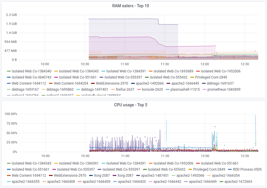
Here's the graph for that section [click to enlarge]:

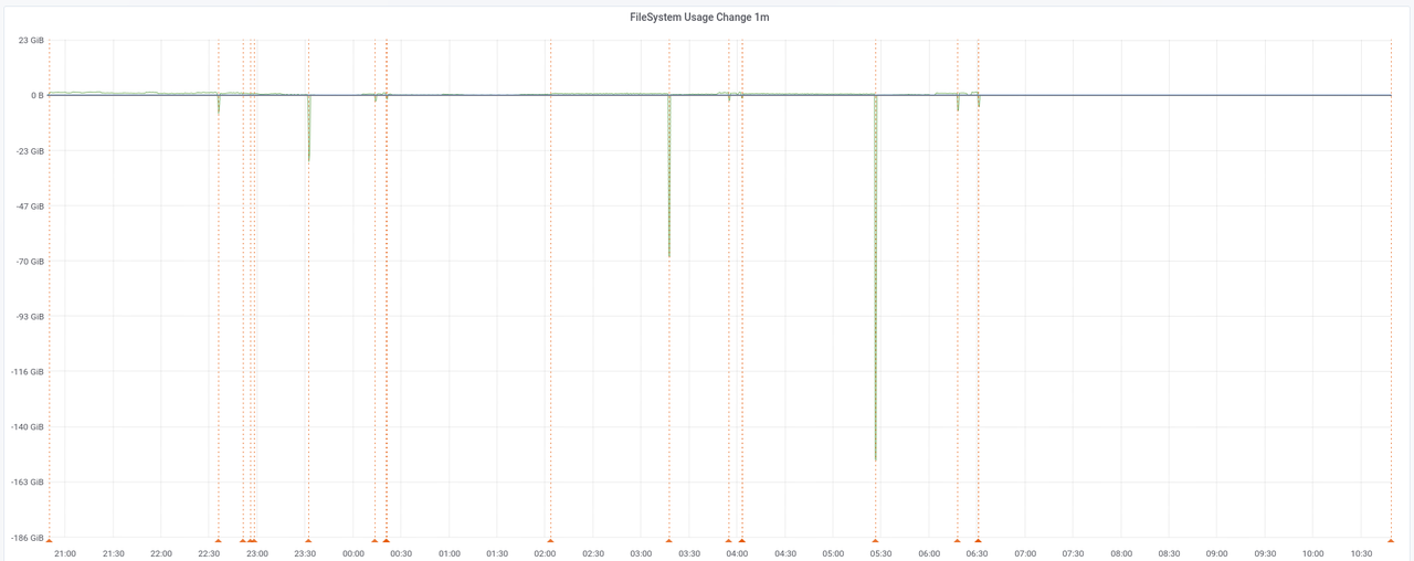
If you look closer, you can barely see the indexes being created, but the most popping up features are the peaks of space being freed. These correspond to points were some task has just finished and another one begins. Correlating back with those logs, and taking just the 4 bigger ones, we get (in chronological order):

  • Clustering the roads table frees 10GiB.
  • Clustering the point table frees 24GiB.
  • Clustering the line table frees 68GiB.
  • Clustering the polygon table frees 153GiB.

Which makes a lot of sense. But there's nothing for us here if we want to reorder stuff because they're all started in parallel, and we could only reorder them if we set --number-processes 1. The space being freed more or less corresponds (at least in terms of orders of magnitude) to the sizes of the final tables we see above. These are also the main rendering tables. The rest is space freed when finishing creating indexes, but the amounts are so small that I'm not going to focus on them. Also, notice that most of the space is freed after the last of those four events because the original data is bigger and so it takes longer to process.

As a side note, I generated the above graphs using Prometheus, Grafana and its annotations. One of the good things about Grafana is that it has an API that allows you to do a lot of stuff (but surprisingly, not list Dashboards, although I guess I could use the search API for that). I tried to do it with Python and requests but for some reason it didn't work3:

Update: the mistake was using requests.put() instead of requests.post(). Another consequence of writing for hours until late at night.

#! /sur/bin/env python3
import requests
import datetime
time = datetime.datetime.strptime('2023-08-18 15:46:20', '%Y-%m-%d %H:%M:%S')
# also tried dashboardId=1
data = dict(dashboardUID='fO9lMi3Zz', panelId=26, time=time.timestamp(), text='Setting up tables')
# Update: not put(), post()!
# requests.put('http://diablo:3000/api/annotations', json=data, auth=('admin', 'XXXXXXXXXXXXXXX'))
# <Response [404]>
requests.post('http://diablo:3000/api/annotations', json=data, auth=('admin', 'XXXXXXXXXXXXXXX'))
# <Response [200]>

I left finding out why for another time because I managed to do the annotations with curl:

$ python3 -c 'import datetime, sys; time = datetime.datetime.strptime(sys.argv[1], "%Y-%m-%d %H:%M:%S"); print(int(time.timestamp()) * 1000)' '2023-08-20 10:48:18'
1692521298000
$ curl --verbose --request POST --user 'admin:aing+ai3eiv7Aexu5Shi' http://diablo:3000/api/annotations --header 'Content-Type: application/json' \
    --data '{ "dashboardId": 1, "panelId": 26, "time": 1692521298000, "text": "Done task [Building index on table planet_osm_ways]" }'

(Yes. All annotations. By hand. And double-checked the next day, because I was doing them until so late I made a few mistakes.)

Here are the indexes this step creates and their sizes:

                    Name                     |                Table                | Access method |    Size
---------------------------------------------+-------------------------------------+---------------+----------------
 planet_osm_ways_nodes_bucket_idx            | planet_osm_ways                     | gin           | 11_817_369_600
 planet_osm_polygon_way_idx                  | planet_osm_polygon                  | gist          | 11_807_260_672
 planet_osm_ways_pkey                        | planet_osm_ways                     | btree         |  8_760_164_352
 planet_osm_polygon_osm_id_idx               | planet_osm_polygon                  | btree         |  6_186_663_936
 planet_osm_point_way_idx                    | planet_osm_point                    | gist          |  4_542_480_384
 planet_osm_line_way_idx                     | planet_osm_line                     | gist          |  4_391_354_368
 planet_osm_line_osm_id_idx                  | planet_osm_line                     | btree         |  2_460_491_776
 planet_osm_point_osm_id_idx                 | planet_osm_point                    | btree         |  2_460_352_512
 planet_osm_rels_parts_idx                   | planet_osm_rels                     | gin           |  2_093_768_704
 planet_osm_roads_way_idx                    | planet_osm_roads                    | gist          |    291_995_648
 planet_osm_rels_pkey                        | planet_osm_rels                     | btree         |    153_853_952
 planet_osm_roads_osm_id_idx                 | planet_osm_roads                    | btree         |    148_979_712
 spatial_ref_sys_pkey                        | spatial_ref_sys                     | btree         |        212_992

Even when the sizes are quite big (51GiB total), it's below the peak extra space (124GiB), so we can also ignore this.

Then it's time to create some indexes with an SQL file provided by osm-carto. psql does not print timestamps for the lines, so I used my trusty pefan script to add them2:

$ time psql --dbname gis --echo-all --file ../../osm-carto/indexes.sql | pefan -t
2023-08-22T21:08:59.516386: -- These are indexes for rendering performance with OpenStreetMap Carto.
2023-08-22T21:08:59.516772: -- This file is generated with scripts/indexes.py
2023-08-22T21:08:59.516803: CREATE INDEX planet_osm_line_ferry ON planet_osm_line USING GIST (way) WHERE route = 'ferry' AND osm_id > 0;
2023-08-22T21:10:17.226963: CREATE INDEX
2023-08-22T21:10:17.227708: CREATE INDEX planet_osm_line_label ON planet_osm_line USING GIST (way) WHERE name IS NOT NULL OR ref IS NOT NULL;
2023-08-22T21:13:20.074513: CREATE INDEX
2023-08-22T21:13:20.074620: CREATE INDEX planet_osm_line_river ON planet_osm_line USING GIST (way) WHERE waterway = 'river';
2023-08-22T21:14:41.430259: CREATE INDEX
2023-08-22T21:14:41.430431: CREATE INDEX planet_osm_line_waterway ON planet_osm_line USING GIST (way) WHERE waterway IN ('river', 'canal', 'stream', 'drain', 'ditch');
2023-08-22T21:16:22.528526: CREATE INDEX
2023-08-22T21:16:22.528618: CREATE INDEX planet_osm_point_place ON planet_osm_point USING GIST (way) WHERE place IS NOT NULL AND name IS NOT NULL;
2023-08-22T21:17:05.195416: CREATE INDEX
2023-08-22T21:17:05.195502: CREATE INDEX planet_osm_polygon_admin ON planet_osm_polygon USING GIST (ST_PointOnSurface(way)) WHERE name IS NOT NULL AND boundary = 'administrative' AND admin_level IN ('0', '1', '2', '3', '4');
2023-08-22T21:20:00.114673: CREATE INDEX
2023-08-22T21:20:00.114759: CREATE INDEX planet_osm_polygon_military ON planet_osm_polygon USING GIST (way) WHERE (landuse = 'military' OR military = 'danger_area') AND building IS NULL;
2023-08-22T21:22:53.872835: CREATE INDEX
2023-08-22T21:22:53.872917: CREATE INDEX planet_osm_polygon_name ON planet_osm_polygon USING GIST (ST_PointOnSurface(way)) WHERE name IS NOT NULL;
2023-08-22T21:26:36.166407: CREATE INDEX
2023-08-22T21:26:36.166498: CREATE INDEX planet_osm_polygon_name_z6 ON planet_osm_polygon USING GIST (ST_PointOnSurface(way)) WHERE name IS NOT NULL AND way_area > 5980000;
2023-08-22T21:30:00.829190: CREATE INDEX
2023-08-22T21:30:00.829320: CREATE INDEX planet_osm_polygon_nobuilding ON planet_osm_polygon USING GIST (way) WHERE building IS NULL;
2023-08-22T21:35:40.274071: CREATE INDEX
2023-08-22T21:35:40.274149: CREATE INDEX planet_osm_polygon_water ON planet_osm_polygon USING GIST (way) WHERE waterway IN ('dock', 'riverbank', 'canal') OR landuse IN ('reservoir', 'basin') OR "natural" IN ('water', 'glacier');
2023-08-22T21:38:54.905074: CREATE INDEX
2023-08-22T21:38:54.905162: CREATE INDEX planet_osm_polygon_way_area_z10 ON planet_osm_polygon USING GIST (way) WHERE way_area > 23300;
2023-08-22T21:43:20.125524: CREATE INDEX
2023-08-22T21:43:20.125602: CREATE INDEX planet_osm_polygon_way_area_z6 ON planet_osm_polygon USING GIST (way) WHERE way_area > 5980000;
2023-08-22T21:47:05.219135: CREATE INDEX
2023-08-22T21:47:05.219707: CREATE INDEX planet_osm_roads_admin ON planet_osm_roads USING GIST (way) WHERE boundary = 'administrative';
2023-08-22T21:47:27.862548: CREATE INDEX
2023-08-22T21:47:27.862655: CREATE INDEX planet_osm_roads_admin_low ON planet_osm_roads USING GIST (way) WHERE boundary = 'administrative' AND admin_level IN ('0', '1', '2', '3', '4');
2023-08-22T21:47:30.879559: CREATE INDEX
2023-08-22T21:47:30.879767: CREATE INDEX planet_osm_roads_roads_ref ON planet_osm_roads USING GIST (way) WHERE highway IS NOT NULL AND ref IS NOT NULL;
2023-08-22T21:47:41.250887: CREATE INDEX

real    38m41,802s
user    0m0,098s
sys     0m0,015s

The generated indexes and sizes:

                    Name                     |                Table                | Access method |       Size
---------------------------------------------+-------------------------------------+---------------+----------------
 planet_osm_polygon_nobuilding               | planet_osm_polygon                  | gist          |  2_314_887_168
 planet_osm_line_label                       | planet_osm_line                     | gist          |  1_143_644_160
 planet_osm_polygon_way_area_z10             | planet_osm_polygon                  | gist          |    738_336_768
 planet_osm_line_waterway                    | planet_osm_line                     | gist          |    396_263_424
 planet_osm_polygon_name                     | planet_osm_polygon                  | gist          |    259_416_064
 planet_osm_polygon_water                    | planet_osm_polygon                  | gist          |    188_227_584
 planet_osm_roads_roads_ref                  | planet_osm_roads                    | gist          |    147_103_744
 planet_osm_point_place                      | planet_osm_point                    | gist          |    138_854_400
 planet_osm_roads_admin                      | planet_osm_roads                    | gist          |     47_947_776
 planet_osm_polygon_way_area_z6              | planet_osm_polygon                  | gist          |     24_559_616
 planet_osm_line_river                       | planet_osm_line                     | gist          |     17_408_000
 planet_osm_polygon_name_z6                  | planet_osm_polygon                  | gist          |     13_336_576
 planet_osm_roads_admin_low                  | planet_osm_roads                    | gist          |      2_424_832
 planet_osm_polygon_military                 | planet_osm_polygon                  | gist          |        925_696
 planet_osm_line_ferry                       | planet_osm_line                     | gist          |        425_984
 planet_osm_polygon_admin                    | planet_osm_polygon                  | gist          |         32_768

The sizes are small enough to ignore.

The last step is to import external data2:

mdione@diablo:~/src/projects/osm/data/osm$ time ../../osm-carto/scripts/get-external-data.py --config ../../osm-carto/external-data.yml --data . --database gis --port 5433 --username $USER --verbose 2>&1 | pefan.py -t '%Y-%m-%d %H:%M:%S'
2023-08-22 23:04:16: INFO:root:Checking table simplified_water_polygons
2023-08-22 23:04:19: INFO:root:  Importing into database
2023-08-22 23:04:20: INFO:root:  Import complete

2023-08-22 23:04:21: INFO:root:Checking table water_polygons
2023-08-22 23:06:16: INFO:root:  Importing into database
2023-08-22 23:07:12: INFO:root:  Import complete

2023-08-22 23:07:49: INFO:root:Checking table icesheet_polygons
2023-08-22 23:07:55: INFO:root:  Importing into database
2023-08-22 23:07:59: INFO:root:  Import complete

2023-08-22 23:08:01: INFO:root:Checking table icesheet_outlines
2023-08-22 23:08:06: INFO:root:  Importing into database
2023-08-22 23:08:09: INFO:root:  Import complete

2023-08-22 23:08:11: INFO:root:Checking table ne_110m_admin_0_boundary_lines_land
2023-08-22 23:08:12: INFO:root:  Importing into database
2023-08-22 23:08:13: INFO:root:  Import complete

real    3m57,162s
user    0m36,408s
sys     0m15,387s

Notice how this time I changed pefan's -t option to have more consistent timestamps. The generated indexes are:

                Name                 | Persistence | Access method |       Size
-------------------------------------+-------------+---------------+----------------
 water_polygons                      | permanent   | heap          |  1_201_078_272
 icesheet_outlines                   | permanent   | heap          |     83_951_616
 icesheet_polygons                   | permanent   | heap          |     74_571_776
 simplified_water_polygons           | permanent   | heap          |     34_701_312
 ne_110m_admin_0_boundary_lines_land | permanent   | heap          |        139_264
 external_data                       | permanent   | heap          |         16_384

                    Name                     |                Table                | Access method |      Size
---------------------------------------------+-------------------------------------+---------------+---------------
 icesheet_outlines_way_idx                   | icesheet_outlines                   | gist          |     3_325_952
 icesheet_polygons_way_idx                   | icesheet_polygons                   | gist          |       679_936
 simplified_water_polygons_way_idx           | simplified_water_polygons           | gist          |       630_784
 water_polygons_way_idx                      | water_polygons                      | gist          |       630_784
 ne_110m_admin_0_boundary_lines_land_way_idx | ne_110m_admin_0_boundary_lines_land | gist          |        24_576
 external_data_pkey                          | external_data                       | btree         |        16_384

Again, too small to care.

Let's summarize what we have.

We started with a 28GiB Europe export, which generated 298GiB of data and indexes, with a peak of 422GiB of usage during the clustering phase. This 'data and indexes' includes an 83GiB flat nodes file, which I need to use because of the puny size of my rendering gig. This means a 10x explosion on data size, but also a 15x peak usage (ballpark figures). As the peak happens in a part of the process that can't be reordered, any other reordering in data import or index generation would provide no advantage. Maybe only if you used --number-processes 1, and given how the clustering of tables are assigned to workers, I think it's already the right order, except maybe swapping the last two, but they're also the smaller two; polygons was already the peak.


  1. psql uses pg_catalog.pg_size_pretty() to print tables and indexes sizes, and it's hard coded on the query that it runs. Thanks to the people at #postgresql:libera.chat I found out that most of the slash commands (for instance, both \d+ and \di+ I used above) are implemented with SQL queries. You can find out which queries by using \set ECHO_HIDDEN 1 and running them again. I sorted them by decreasing size, and I used Python's long int prettifying method :) I also removed uninteresting columns. 

  2. I removed lines from this output that I think don't add new interesting info, and I split it in sections so it's easier to read and marks important milestones for the graphs later. 

  3. I usually use a highlighter for these snippets, but alas, it's broken right now. I've been kicking down the road a migration out of ikiwiki to probably nikola, maybe it's time. 

Deploying venv based Python services with Ansible and systemd

Today I deployed my first venv based python system service on my home server. This is a short post describing how I did it.

One of the hardest problems in Computer Science is naming :) In this particular case, where to put the code. Initially I thought of something like /usr/local/lib/python<version>/site-packages/something/<app>, but frankly only because I have completely forgotten about /opt, even when I was dealing with it daily no more than 3 months ago. So /opt/<app> it is.

Next came automating all the right steps. I install everything on that server with Ansible. It's weird to write down all the steps when one's used to do them by hand. This includes:

  • Create the dir
  • Copy the files
  • Create the venv
  • Install deps
  • Install the systemd service file

The way Ansible works, you can tell it not to repeat tasks if you tell it which files it creates. The way venvs work in python, they're created on a dir that contains the major and minor python version: <venv_dir>/lib/python<version>. To avoid creating the venv on every Ansible run, I need the Python version, but just those two components. After some testing and sharing and being corrected, I got this:

python3 -c 'import sys; print(".".join(map(str, sys.version_info[0:2])))'

map(str, ...) is needed because join() expects a list of strings.

Another thing you can do with Ansible is to emit events that can make handlers (another type of tasks) run. In this case this is useful to restart the service if the code or the config changes, but also to refresh systemd if the service file changes.

This is the first time I used a feature of venvs. venvs contain in their bin directory several scripts. The most important for me so far was the bin/activate environment file. If you source it, it will set up PATHs properly so Python can find the deps within the venv. But it also creates a python3 and pip3 scripts that run both tools also with the PATHs modified. This simplifies many things when manipulating venvs with Ansible, and also systemd.

The last link is on the systemd side. I didn't really want to install everything neatly in /opt and then put the service file outside it. systmctl link exists exactly for that. It creates a link in /etc/systemd/system to the service file in /opt. It's still not 100% clean, but at least it's managed by systemd, and you can clearly see who really owns it. You run this command instead of systemd enable, and it's ready for starting it.

Here's the whole play:

- name: Apache Log Exporter  # this one has its own play because it's more complex than the rest
  hosts: servers
  tasks:
  - name: Create dirs
    file:
      path:  /opt/apache-log-exporter
      state: directory
      owner: root
      group: root
      mode:  0755
    tags: install, monitoring

  - name: Install PALE bin and conf
    template:
      src:   "roles/server/files/{{ item }}"
      dest:  "{{ item }}"
      owner: prometheus
      group: root
      mode:  0600
    loop:
      - /opt/apache-log-exporter/apache-log-exporter.py
      - /opt/apache-log-exporter/apache-log-exporter.yaml
    tags: install, config, monitoring
    notify:
      - Reload Apache Log Exporter

  - name: Install PALE service
    template:
      src:   "roles/server/files/{{ item }}"
      dest:  "{{ item }}"
      owner: prometheus
      group: root
      mode:  0644
    register: pale_service
    loop:
      - /opt/apache-log-exporter/apache-log-exporter.service
    tags: install, config, monitoring

  - name: Get Python Version
    # thanks @diji@mastodon.social
    command: python3 -c 'import sys; print(".".join(map(str, sys.version_info[0:2])))'
    register: python3_version
    tags: install, monitoring

  - name: Create PALE VEnv
    command: python3 -m venv --prompt pale --system-site-packages venv
    args:
      chdir:   /opt/apache-log-exporter
      creates: "/opt/apache-log-exporter/venv/lib/python{{ python3_version.stdout_lines[0] }}"
    tags: install, monitoring

  - name: Install PALE Deps
    command: "/opt/apache-log-exporter/venv/bin/pip3 install {{ item }}"
    args:
      creates: "/opt/apache-log-exporter/venv/lib/python{{ python3_version.stdout_lines[0] }}/site-packages/{{ item }}"
    loop:
      - apachelogs
      - prometheus_client
    tags: install, monitoring

  - name: Install PALE service
    command: systemctl link /opt/apache-log-exporter/apache-log-exporter.service
    when: pale_service.changed
    tags: install, monitoring
    # systemctl link already tells systemd about the new file, but we need to restart the service
    # notify:
    #   - Reload Systemd

  handlers:
  - name: Reload Apache Log Exporter
    service:
      name:  apache-log-exporter
      state: restarted

  - name: Reload Systemd
    command: systemctl daemon-reload

The systemd unit file also uses the venv scripts:

[Unit]
Description=Apache-Log-Exporter
Wants=network-online.target
After=network-online.target

[Service]
Type=simple
User=prometheus
Group=prometheus
ExecStart=/opt/apache-log-exporter/venv/bin/python3 -u /opt/apache-log-exporter/apache-log-exporter.py --config-file /opt/apache-log-exporter/apache-log-exporter.yaml
Restart=always
RestartSec=10s
NotifyAccess=all

[Install]
WantedBy=multi-user.target

Apt lists lock held by python

In my laptop I run Debian Sid. A long time ago I decided to update it only on Sundays afternoon, so if any bugs that might have appeared during the week would have most probability of being either known or already fixed (but probably also means that more bugs can be introduced, assuming Debian Developers work mostly during weekends, so...). I mostly use aptitude but if I have to be honest, I miss the dependency dialogs from dselect: when you selected a package with missing dependencies, a new window showing the automatically added dependencies and also the Recommends and Suggests (mostly because I configured it so Recommends were not selected automatically).

Yesterday I forgot to do the upgrade, so I tried it today. To my surprise, I got this error:

┌────────────────────────────────────────────────────────────────────────────────────────┐
E: Could not get lock /var/lib/apt/lists/lock. It is held by process 2415644 (python3) ▒│
W: Be aware that removing the lock file is not a solution and may break your system.   ▒│
E: Unable to lock directory /var/lib/apt/lists/                                        ▒│
                                         [ Ok ]                                         
└────────────────────────────────────────────────────────────────────────────────────────┘

I checked all my open terminals for any stray apt or aptitude running, but I didn't find any. Then I realized it was talking about a python3 process, but both tools are developed in C++. Who's the culprit?

$ ps faux | grep -C 5 2415644
root     2415643  0.0  0.0   9468  3500 ?        Ss   13:04   0:00 /bin/bash -c /usr/share/prometheus-node-exporter-collectors/apt_info.py | sponge /var/lib/prometheus/node-exporter/apt.prom
root     2415644  0.5  0.2  90600 76512 ?        S    13:04   0:00  \_ python3 /usr/share/prometheus-node-exporter-collectors/apt_info.py
_apt     2415651  0.0  0.0  27652 12856 ?        S    13:04   0:00  |   \_ /usr/lib/apt/methods/https
_apt     2415652  0.0  0.0  27628 12820 ?        S    13:04   0:00  |   \_ /usr/lib/apt/methods/https
_apt     2415653  0.0  0.0  17452  5840 ?        S    13:04   0:00  |   \_ /usr/lib/apt/methods/file
_apt     2415654  0.0  0.0  24400  9564 ?        S    13:04   0:00  |   \_ /usr/lib/apt/methods/https
_apt     2415655  0.0  0.0  27624 12972 ?        S    13:04   0:00  |   \_ /usr/lib/apt/methods/https

prometheus-node-exporter-collectors runs every 15m and locks the db. So this is a transient error, although it doesn't go away very quickly. I think I tried 2 or 3 times, then I started writing this post, then I tried again and it worked. Good to know.

Webmail with roundcube, postfix and dovecot

Note: the coherence in this post is not my usual level, mostly because it's an edit of something I dictated to my phone and later transcripted with whisper. Rambling to a phone for 15m is not the same as sitting down a couple of hours to write. So pardon for the apparent incoherence.

I have had the same email account for more than 20, maybe 25 years, and this account lives in a computer that used to be an important computer at the university, but now it's just a VM. That means that all my personal emails goes to a computer that cannot really handle all the volume I have accumulated in those 20, 25 years. To cope with that I've been fetching all the emails into my personal laptop at home, and then do a backup to my home server. That way I always have all the email in my computer.

But lately I'm not so much at my computer as I used to be as before. To start with, I don't work on that computer like I used to, and also I have less computer time than before (kids, family, friends, other activities). That means that most of the time I cannot read my email because it's stuck in a mutt session on my laptop at home. What I do have most of the time with me is my phone, so what can I do to make my phone be able to reach those emails at home? And even sometimes I don't even have my phone, and I only have someone else's computer. How can I reach my emails there?

The solution is not so simple, but it involves this home server that I have. The idea is to set up an email server on it that will do basically four different things. One of them will be to fetch all the emails from the small server, my personal computer will not do that anymore. Second, it will have a SMTP server that will have that VM as a smart host, and forward all emails to it. Third, it will provide an IMAP server that will serve all those emails, and fourth, it will provide a webmail interface.

That home server is running Debian, so that means that I will preferably install things via packages, and luckily, most of the software is already available. For the SMTP server I will use Postfix, for the IMAP server I will use Dovecot, and finally for the webmail I will use RoundCube.

The first thing I set up was Postfix, and it was quite easy. I started by configuring it with dpkg-reconfigure -p low postfix so it would ask all the questions about the email setup. It was not good enough because I needed to authenticate to the smart host, so there was some further configuration on that, but it's very well documented, so it was easy to do.

The second part was the IMAP server, and it was also very easy. Dovecot does not ask you anything at install time, but the configuration is quite easy, especially when you use PAM authentication. Once I had Dovecot running with authentication, I connected Postfix to Dovecot to do authentication. It was also easy to use the Let's Encrypt certificates with both services.

Then it came to the time to do RoundCube. Installing it was quite easy. Doing IMAP was quite easy too, especially because it's not using the IMAPS port, but only the IMAP port via localhost. Then it came the time to configure it to send email. Initially Postfix was doing SMTP and submission without authentication and RoundCube by default uses it, and it was complaining when the AUTH capability was not being offered before switching to TLS:

 SMTP server does not support authentication

I didn't have authentication on Postfix, so I configured Postfix with Dovecot, and it worked on the phone (K9 on Android), but on RoundCube it still refused to work. Asking in #postfix@libera.chat people told me that AUTH will not appear until the client turned on TLS, which RoundCube didn't seem to be doing, so I decided that I would rather have implicit encryption instead. I turned off SMTP and submission and turned on submissions on Postfix. K9 connected to it fine, but RoundCube still refused, now with these messages:

 PHP Error: Failed to connect socket: Connection refused
 SMTP Error: Connection failed:  (Code: -1)

Anyone used to developing clients know that Connection refused means the port is not available, either because nothing is listening there or because there's a firewall, but the port was open and there was no firewall involved; and, again, K9 connected just fine. I even stopped apache2 and run strace apache -X while turning on debugging logs in Postfix and I could actually see RoundCube properly connect but issue a QUIT command right after connection.

RoundCube makes a little bit of a mess with the configuration around encryption. There's a setting that is called smtp_host; at least that's how Debian writes config.inc.php. In that setting you have to put the address or the name of the server that RoundCube should use for sending emails. If you don't put any protocol in the URI, it will assume the protocol is SMTP. The second option is using explicit encryption with StartTLS. Unluckily the RoundCube decided to use tls:// as the protocol for that. The third option, which is called implicit encryption, is currently using TLS, which superseeded SSL, but RoundCube's protocol for that is ssl:// and not tls://.

That's the first source of confusion; the second source of confusion is that the Debian configuration file lists the setting as smtp_host, but if you check RoundCube's documentation, it's smtp_server. In fact, RoundCube seems to accept both, but when you're writing the configuration file and reading documentation at the same time, it's just confusing.

Debian by default uses tls://localhost:576, and confused with the TLS/SSL thing explained before, I changed it to tls://localhost:465. Once I figured the TLS/SSL thing, I used ssl://localhost:465, but still no cigar. By this time I was in the ##email@libera.chat IRC channel, and someone pointed out that it was maybe the fact that the Let's Encrypt certificate does not cover localhost. And that was it, I changed the URI to point to the FQDN of the certificate and it worked.

To be honest, when K9 connected to both IMAP and submissions, it complained about the cert (I was connecting via IP), but I told it to ignore that. RoundCube, instead, just complained it couldn't connect and lead me into the wrong rabbit hole.

My main email workflow will continue to be through my laptop, so the next step is to synchronize my laptop emails with the server. mbsync in the isync package seems to be the answer, but that's a story for another time.

Unintuitive expressions

One of the aphorisms of the Zen of Python says:

Explicit is better than implicit.

Go dehl writes this code to solve FizzBuzz:

for i in range(1, 101):
    print('FB' if not i % 15 else 'F' if not i % 3 else 'B' if not i % 5 else i)

Read that expression out loud: “the string 'FB' If not i modulus 15; else 'F' if no i modulus 3; else 'B' if not i modulus 5; else i”. It sounds exactly like the opposite of the solution! Why? Because Go dehl is (ab)using the fact that 0 is false-y. A number a is a multiple of another number b if a % b is 0, and 0 evaluates to False in boolean context1, so he's negating that instead of writing if i % 15 == 0 . It's a tendency that I also see in other languages where they write a && b instead of if a: b. Sometimes we get used to these shorthands, but in this case, to me, it was completely confusing. So, please, “Explicit is better than implicit”.

I would have written this as a comment on their blog, but it only works if I login with a Google account, which I don't have; hence, this post.

Encoding and decoding errors

I was bored and I thought this could be useful, not only for you, but for me too.

So you have this text:

 sáb

What happened there? This is a classic encoding error. In fact, it's one of the classic encoding errors. That text is supposed to be 'sáb', but somehow somebody got the bytes all wrong. How wrong? This way.

As Python's Unicode HOWTO1 explains, texts are encoded using encodings so they can be written in a file or sent via network. The problem arises because bytes alone don't have information of the encoding that was used, and those receiving or reading the bytes might need to guess.

One way to solve this is to make the data format to carry that info. That's exactly what your Python files should have at the very beginning:

# -*- coding: utf-8 -*-

In particular, the Pyhton interpreter reads your file first as bytes, searches for such string in the first two lines, and if it finds it, uses that encoding to decode your file. Otherwise, it just guesses that's your system's encoding and prays he got it right2.

HTML files have something similar. They can declare an encoding in the file, and the browser has to do something similar3:

<meta http-equiv="Content-Type" content="text/html; charset=utf-8" />

So what happened to the text? Encoded text is just a sequence of bytes. Each byte has 8 bits, so it can be any value between 0 and 255. At the same time, one of the encodings, latin1, represents its 256 codepoints as values between 0 and 255. This means that you can decode any arbitrary sequence of bytes as latin1 codepoints, even if the original encoding is more complex, like utf-8. Thay way, you end up with things like this:

In [^28]: 'sáb'.encode().decode('latin1')
Out[^28]: 'sáb'

This is probably both the most common decoding error and the easiest to recognize, mostly because of Ã, or because strings are longer than they should (any non-ASCII character is encoded with two or more bytes).

The inverse can happen too, but more infrequently. This is because not any random sequence of bytes is a valid utf-8 encoding. So, SÃO in latin1 is b'S\xc3O', but if you try to decode it to utf-8 you get the most dreaded UnicodeDecodeError, but only because the 3rd byte is below 0x80. But take for instance FORMULÆ®, a reasonable string. Watch this:

In [^17]: bytes('FORMULÆ®', 'latin1')  # there is some mind bending black magick here
Out[^17]: b'FORMUL\xc6\xae'

In [^18]: bytes('FORMULÆ®', 'latin1').decode('utf-8')
Out[^18]: 'FORMULƮ'  # that's a 'LATIN CAPITAL LETTER T WITH RETROFLEX HOOK'

In short, some latin1 sequence of bytes that perfectly decode in utf-8.

There are couple of extra things there. Most of the strings you see here where typed by me either in this editor or on a terminal. How the sequence of keys become bytes in your input is a whole another can of worms, which I don't really have the energy to get into. Maybe some other day. Also, as mentioned in the comment up there, the string FORMULÆ® was typed in utf-8 (or any other encoding I might be running on, but seriously, you should stop using any other), but Python converts that into a unicode string, and then I can perfectly ask bytes() that I want the latin1 representation instead.


  1. https://docs.python.org/3/howto/unicode.html 

  2. If you want to know a little more, let me tell you that just after that, the Python interpreter encodes it to utf-8. I still don't know why. 

  3. The web server also can declare a content encoding with a Content-Type: text/html;coding=utf-8 header. 

Monitoring servers with prometheus and Firefox tabs

I suddenly found myself with a lot of time in my hands, so I decided to play with my home lab, which I hadn't been able to for ages. First stop is monitoring. I already had Prometheus and Grafana installed, with a few dashboards and panels running. I also had Munin, which is an old school, mostly static monitoring system, but which, at least in Debian, has a lot of scrapers builtin. Debian's postinstall script checks your system and enables all the relevant ones, so you get a lot of 'panels' out of the box. The plan was to try to mimic some of Munin graphs with Prometheus and Grafana.

I first attacked one of the most complex ones, which is the memory graph, with 13 metrics on it. All the data comes directly from the node exporter, and most lines are just picking a metric. The only calculated values are swap usage (node_memory_SwapTotal_bytes - node_memory_SwapFree_bytes) and app usage (node_memory_MemTotal_bytes - node_memory_Buffers_bytes - node_memory_Cached_bytes - node_memory_Shmem_bytes - node_memory_PageTables_bytes - node_memory_Slab_bytes - node_memory_MemFree_bytes). Graph wise you have to stack the metrics, except active, inactive, commited and mapped, and put swap on the top, so they all add up to the available RAM and swap becomes like a 'crest' on top. See how beautiful it is:

The first thing I notice is that sawtooth figure, the classical look of a memory leak, so it's time to go deeper. A tool like htop might give you a clue, but as it's always showing the current status, you can't see trends. On the Prometheus side there's the process exporter, so I installed that; Munin doesn't have anything like it, so you'll have to search for one, but it would probably be shorter to write your own. I configured the PE to monitor all processes (there are only ~250 running at a time), using the process name and PID as name (name: "{{.Comm}}-{{.PID}}"). Then I fire up a new panel that graphs topk(10, namedprocess_namegroup_memory_bytes{memtype="resident"}), the top 10 RAM eaters.

And sure enough, 2 Firefox subprocesses are the top culprits. This machine is both my home server and the media center, and being a single parent now means that the kids watch TV while I do the chores (cooking, mostly; the rest are done when they're sleeping). So, Firefox is always up with 2 or 3 tabs (among the usual loitering tabs one always has around waiting to be read, which almost never happens) where they watch their favorite content. Maybe these tabs are constantly accumulating data from the sites, and maybe at some point Firefox is reaping them because they're taking too much RAM. To test the theory, I closed one of the tabs, but instead of one of those processes disappearing as I expected, one just reduced considerably its resident size.

I waited a while, closed a second one, an the process disappeared from the top 10, meaning it went from 1.9GiB to less than 105MiB of resident size! I'm not going to name the culprit, suffice to say it's a streaming service with an Irish name. I had also setup a Top 5 CPU users, and sure enough, by the time I closed this second tab, its CPU usage went from a jumpy 3-50% to a stable 3%. So far so good!

But there was a second Firefox process using RAM and CPU. Which tab could this be? There were still a couple of tabs with often used streaming services open, but can we try to investigate which ones are tied to this process? Looking around I found about about:processes instead, which is not exactly what I was looking for, but it was good enough to figure out that it was not a streaming site but a news one. Again no names, I'm just going to say it's a sibling of the site that went bankrupt over a sex tape. It was a good thing I tried to get the facts right instead of trying to close tabs blindly!

Unluckily, there doesn't seem to be a way to get this info from outside Firefox, so for now I'll just have to be conscious about the tabs that are left open. This is how these two graphs look now:

Blender hillshading and mapnik

How did it start? Well, it actually started a long time ago, maybe a year ago, most probably more. I got myself tumbling down the beautiful rabbit hole of Blender based mapping. The idea is very simple: if you have a DEM, you can build a 3D representation of the terrain and use a renderer to build your map. To me the most striking thing about those maps were not their 3D-ness (which to some it's starting to be tiresome , and I agree), but the shadows. I've been pursuing the best shadow for a while, and this seemed like the perfect fit.

So, like I said, one year ago or so I took "the" Blender relief tutorial and run with it. I got to the point where I could reproduce it with a 1x1, 3600x3600px DEM from mapzen, but when I tried to automate it, I found out that Blender has a python console where it prints out the commands that are equivalent to the actions you make in the UI, but the resulting script was too horrible to my eyes and run out of breath (another of those cases of the perfect being the enemy of the good).

Then a few days ago I read that first link and got some steam build up. In fact, it was two passages in it that lit up the fire:

Most of these use a tool called Blender, an extremely powerful open-source tool for all kinds of 3D modeling and rendering. A few cartographers use other tools, such as Aerialod, or R‘s Rayshader plugin.

R! I can easily automate this!

If we stick to a very zoomed-out map, or if we have a really huge computer running Blender, we could try to do a hillshade for the entire world, and then slice that up for our map tiles. But there’s no way we could do this at a high-enough resolution so you could zoom all the way in, as in the sample tiles above.

Challenge accepted! (Spoiler: I'm not there yet).

I tried Rayshader. I wanna be honest: it's easy, quick, but I didn't like the results. It seemed like no matter how high you put the sun, it always drew very long shadows. So despite its pragmaticism, I left it on a side.

So I picked up what I did in the past and tried to apply it to a map. I re-rendered everything and applied it to my style. The outcome was encouraging:

To start with, I probably did that render with not enough render passes, so the output looks grainy. Second, the material color is too bright, so the height tints are washed out. Still, we can see the big shadow cast over the valley some 3200m below the Mont Blanc/Monte Bianco.

This proved to be a good place to test the method, because of the great difference between the valley and the peak casting the shadow over it, and that lead me to think: are there more extreme places in the world? An easy bet is yes, and the place to look for them was the Himalayas. The Aconcagua could have been a good contender, but the valley at its SE is some 4550m already. Surprisingly, the way I searched for a good place was to use existing maps with the usual hill shade technique, looking for big dark spots, specially those wide in the NW-SE direction. I first found my spot in the Tukuche Peak, that looms some 4350m above the Gandaki River, and then the nearby Dhaulagiri, that's even some 1250m higher, clocking at 8167m. Here's how they look (not the big structure in the upper left, but the bigger grey [8000m+] blob to the East of it; the river snakes in the right all the way down):

I had to add 3 more color bands to my style and reshuffle them because I never rendered any 8k'er before, so the colors were haphazardly concocted for the rendering and are not definitive. At least it lets you behold the grandiosity of that rock jutting through thousands and thousands of meters with very steep sides.

Time to get real. I usually render regions were I'll be going, and next time it's the Upper Segre Valley, so I rendered N42E001-2 in one go. That's 7201x4884px after reprojecting to WebMercator (and compensating as described in the second link!), so some 35Mpx. Blender took some 44m+ on a 4.5yo medium-high spec'ed laptop at 200 render samples, which means that I can continue to render small regions this way, but that for the moment I won't be applying this technique to the whole Europe.

Up to here I was just applying the same style in QGIS, which has been an indispensable tool to develop this style. But trying these TIFFs in mapnik for the first time needed an extra step. Well, two, in fact. Blender does not save the TIFFs georeferenced, so you have to copy the data from the original DEM. For that, use gdal_edit.py -a_srs ... -a_ullr ... with the right ESPG and the data from the output of gdalinfo. Next, for some reson, it always use 16bits integers, even when explicitly saying to use 8. This little snippet takes care of that:

import imageio

image = imageio.imread('pirinoak-blender-10x.tif')
image = image / 256
image = image.astype('uint8')
imageio.imwrite('pirinoak-blender-10x-8bits.tif', image)

Thank $DEITY (and developers!) for good libraries.

The first thing I noticed was that we have been lied by maps (again!) for a long time. Most hill shading algos use a 45° high sun (the direction does not matter much). But if you think about it, how many mountains have sides 45°+ steep? According to a (real, not like me!) cartographer friend, for continental Argentina it's less than 1% at 30arcsecs of resolution (note that SRTM is 1arcsec). Still, some shadows are there, and they help us (and we get used to that) to recognize slope direction. And now we're asking a raytracing program to calculate real shadows? The result I initially got was underwhelming, even when I was already asking Blender to exaggerate height by 5x!:

So, I bit the bullet and went all in with 10x:

Much better, but not definitive. I still have to render Dhaulagiri again, and at least some region I already know well by having being there a lot. Here's how that region looks in my style:

Now some notes about "the" Blender relief tutorial. I followed it to the letter, but with my experience I had to make some changes. One you already know, using a displacement scale of 10x instead of 0.3. I have no exact idea why his initial rendering were so spiky, but I suspect that the DEM grid unit was not meters.

Second, since that first Mount Blanc/Monte Bianco render, we know the color is too bright. I lowered it to 0.6 (and later I found that that's what he actually suggests at the end of the plane section) and then compared the grey in a plain (#b5b5b5) to what GDAL outputs and compensated using a simple coefficient. The final value is 0.402.

Third, I was having issues rendering: I was getting a lot of terracing. After a long chat with Viktor_smg from blender.chat/support they figured out that the sRGB color space in the Image Texture is broken and that I should use XYZ instead. This meant installing Blender by hand instead of relying on the one in Debian Unstable because it's too old and does not have it. They also gave me pointers about how to automate it.

Last, you can't apply this technique DEM by DEM because you want the shadows from the neighbouring tiles to spill over the current one. That link shows how to render the tile and its 8 neighbouring ones, but I think that you can optimize it in two ways: First, since shadows come from the NW, just add the tiles that lie in that general direction. Second, no shadow would cast over 10s of kilometers. You could even get away with just adding a smaller band around the tile.

That's it for now. The next step is to automate this an publish that. $DEITY knows when that will happen.